Article Text

Abstract
There is an ongoing debate on whether analyses of occupational studies should be adjusted for socioeconomic status (SES). In this paper directed acyclic graphs (DAGs) were used to evaluate common scenarios in occupational cancer studies with the aim of clarifying this issue. It was assumed that the occupational exposure of interest is associated with SES and different scenarios were evaluated in which (a) SES is not a cause of the cancer under study, (b) SES is not a cause of the cancer under study, but is associated with other occupational factors that are causes of the cancer, (c) SES causes the cancer under study and is associated with other causal occupational factors. These examples illustrate that a unique answer to the issue of adjustment for SES in occupational cancer studies is not possible, as in some circumstances the adjustment introduces bias, in some it is appropriate and in others both the adjusted and the crude estimates are biased. These examples also illustrate the benefits of using DAGs in discussions of whether or not to adjust for SES and other potential confounders.
Statistics from Altmetric.com
In recent years there has been increasing interest in the use of directed acyclic graphs (DAGs) to consider issues of adjustment for potential confounders in epidemiological studies.1–3 DAGs are constructed on the basis of a priori assumptions about the causal relationships between the variables of interest. Arrows connecting the variables represent these causal links. If the assumptions hold, then a graphical method following simple rules (called the “d-separation” method) can be used to understand when two variables are conditionally independent.1 4 5 These rules have been formally described previously.1 4–8 Briefly, two variables are statistically independent if all paths connecting the two variables are blocked. Paths are, in Pearl’s 5 words, “any succession of arcs connecting variables, regardless of their directions”. A path is blocked when either (1) two arrowheads on the path converge on the same variable (which is called a “collider”) or (2) a non-collider on the path has been conditioned on. Conversely, conditioning on a collider, or on a descendant of a collider—that is, a variable caused by a collider—opens the path between previously independent causes of the collider. If all paths between an exposure and a disease are blocked then the two variables are d-separated and the structural sources of confounding of the exposure–disease association have been accommodated.
DAGs have been used relatively little to date in discussions of confounder control in occupational studies, even though there are a number of methodological issues that would benefit from the use of DAGs. In particular, for several decades it has been debated whether the reference group in occupational studies should have the same socioeconomic status (SES) as the exposed group,9–13 i.e. whether analyses of occupational studies should be adjusted for SES. The problem arises because occupational factors and SES are strongly associated. If SES is also associated with an increased cancer risk, then it may seem reasonable to adjust for SES as a confounder in the analysis. However, adjustment for SES, or restriction of the comparison group to the same SES as the exposed group, may mean that the comparison group involves a relatively high prevalence of other occupational exposures, which in turn, may be determinants of the cancer under study. For example, if the analysis is restricted to “blue collar” workers, then the comparison group may be exposed to other occupational factors that cause the occupational health outcome under study.9
Similar debates on the relationship between occupation and SES have taken place also in non-cancer contexts. It has been recently argued that SES, in terms of attained education or social prestige and attained economic or political power, should not be treated as a confounder in the analysis of occupational determinants of back morbidity, because components of SES may be surrogates of physical, psychosocial and environmental working conditions.14 15 Under this view, the effects of SES and occupational exposures are inseparable. However, the extent to which this hypothesis is valid will of course vary greatly according to which risk factors and which diseases are being considered. In particular, the difficulties of separating SES from occupation may be much greater when considering chronic musculoskeletal disorders, with variations in exposure, disease status, SES and occupation over time, than when considering cancer incidence which occurs at one point in time. Furthermore, most occupational epidemiologists do attempt to assess the independent contribution of SES and occupational exposures, and when they do, a number of issues arise in that, as noted above, the comparison group may involve a relatively high prevalence of other occupational exposures, which, in turn, may be determinants of the cancer under study.
Although this problem has been recognized for some time, the issues of adjustment for SES in occupational studies have not been investigated in depth. For example, in three leading epidemiological journals (American Journal of Epidemiology, Epidemiology, Cancer Causes and Control) there were 16 original occupational cancer studies (5 cohorts, 6 case–control studies, 4 nested case–control studies, 1 case–cohort study) published in 2005.16–31 Only five used information on SES (either the educational level or the last occupation) in the analysis,16 17 21 22 30 whereas, according to the information reported in the method section of the articles, nine of the remaining 11 studies either had or could have collected information on SES.18–20 23–25 27 28 31 In one of the five studies in which the last occupation was included in the data analysis, the issue of adjustment for SES was briefly discussed and authors decided to present adjusted estimates only.21 In another study only unadjusted estimates were reported in the abstract.16
In the present paper, we use DAGs to evaluate common scenarios in occupational cancer studies, and to clarify under which circumstances adjustment for SES is appropriate.4 32
The association between socioeconomic status and occupational factors
Although occupational status can influence SES, and vice versa, in this paper we will focus on the situation where SES and occupational status are associated because they share common causes. In fact, SES can be measured using a number of possible indicators, such as education, income, household conditions, deprivation and occupation itself.33–35 These “indicators” are more correctly viewed as different, albeit in part overlapping and correlated, aspects of a multidimensional individual characteristic, that is usually summarised as SES and may also include the occupational status.34
In this paper, for simplicity we will not consider issues of random variation (variables that are not structurally associated may be associated by chance in a finite population), decreasing precision with increasing complexity of the models, and measurement errors of the exposure and confounders.4 32
Common scenarios
In this section we will consider the most common and basic scenarios in occupational cancer studies using DAGs and numerical examples. The exposure of interest will be assumed to not be associated with the cancer under study (ie the true relative risk is 1.0).
Scenario 1
Let us assume that a study is conducted to investigate the association between having worked as a waiter (O) and the risk of testicular cancer (D) (fig 1).
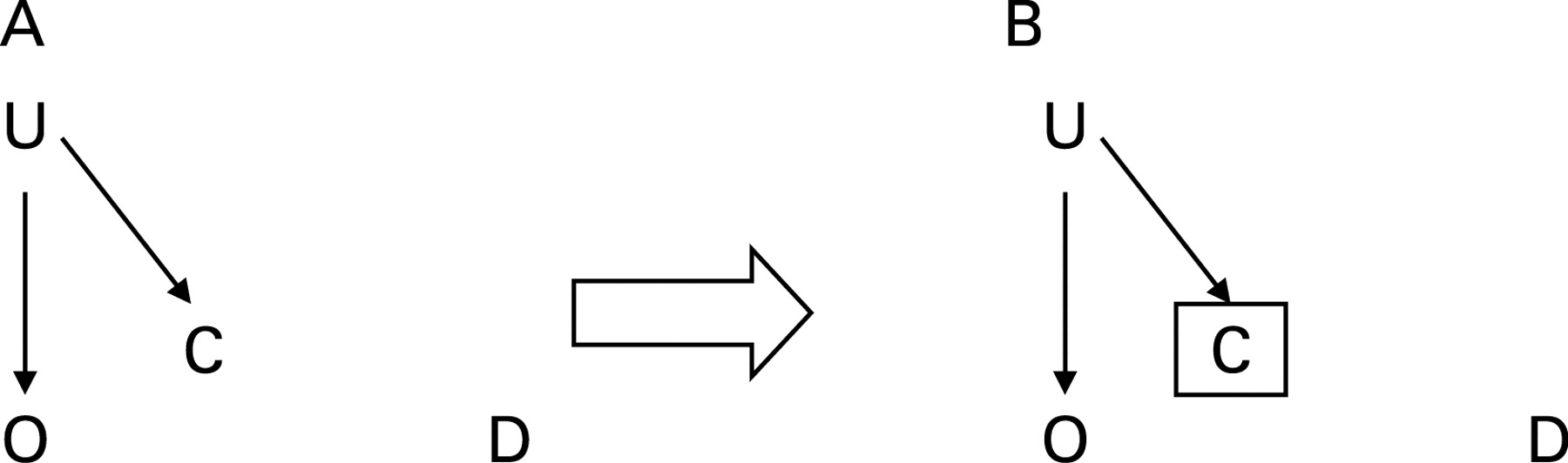
Although an association between SES (C) and testicular cancer risk (D) has been observed in the past, there is evidence that the association has attenuated in recent times.36 Under this simple scenario, having worked as a waiter (O) and SES (C) are associated with each other, but not with cancer risk (D) (fig 1A). Therefore, adjustment for SES (C) would not affect the relative risk (RR) estimate for the association between having worked as a waiter (O) and testicular cancer risk (D) (fig 1b). In fig 1 and throughout the article a square around a variable means conditioning for that variable. Moreover, throughout the article dashed lines without arrowheads are used to connect independent causes of a collider, which has been conditioned on.
Scenario 2
A more complex scenario is the situation of a study investigating whether having worked as a waiter (O) is a risk factor for pleural mesothelioma (D) (fig 2).
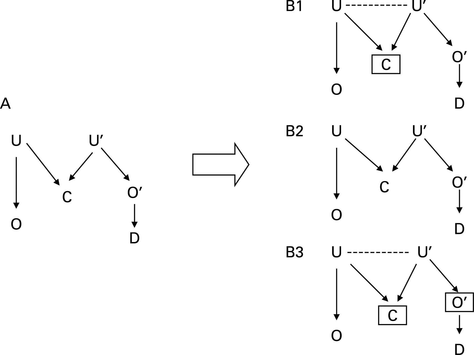
Although SES (C) is not itself a cause of mesothelioma (D), there is a strong association between having a low SES (C) and working in occupations (O′) that entail exposure to asbestos, an established carcinogen of the pleura (fig 2).37
Under this scenario, SES (C) becomes a collider, meaning that two arrowheads on the path collide on it (fig 2A). According to the d-separation method, a path that contains a collider is blocked. It follows that adjustment for SES (C) would open the path, creating a spurious association between having worked as a waiter (O) and mesothelioma risk (D) through exposure to asbestos (O′) (fig 2B1). Conversely, the unadjusted estimate would be valid (fig 2B2). However, if complete information on occupational history (O) is obtained, and exposure to asbestos (O′) can therefore be adjusted for in addition to SES (C), then the path containing asbestos exposure (O′) is blocked and the adjusted analysis is valid (fig 2B3).
The diagram shown in fig 2A is a so-called “M diagram”, and is a classic example of a situation in which adjustment for a factor may introduce bias.4 38 A hypothetical example of a study of mesothelioma risk (D) among waiters (O) is shown in table 1.
In this population, 10% of the individuals worked as a waiter (O), whereas 50% of them worked in occupations entailing exposure to asbestos (O′). The prevalence of low SES (C = low) among occupationally unexposed subjects (O = no and O′ = no) is 30% whereas it is 60% in individuals that either worked as a waiter (O = yes and O′ = no) or were occupationally exposed to asbestos (O′ = yes and O = no), and 84% in those with both exposures (O = yes and O′ = yes). There is no crude association between having worked as a waiter and exposure to asbestos (RROO′ = 1.0). Occupational exposure to asbestos causes a fivefold increased risk of mesothelioma (RRO′D = 5.0), whereas SES is not a determinant of mesothelioma risk (RRCD|O′ = 1.0). When the analysis is stratified on exposure to asbestos (O′) and SES (C), the stratum-specific relative risks are 1.0. Thus, the crude estimate, and the estimate adjusted for SES (C) and asbestos exposure (O′) are both 1.0. However, when adjusting for SES alone the RR is biased downwards (RROD|C = 0.9).
Scenario 3
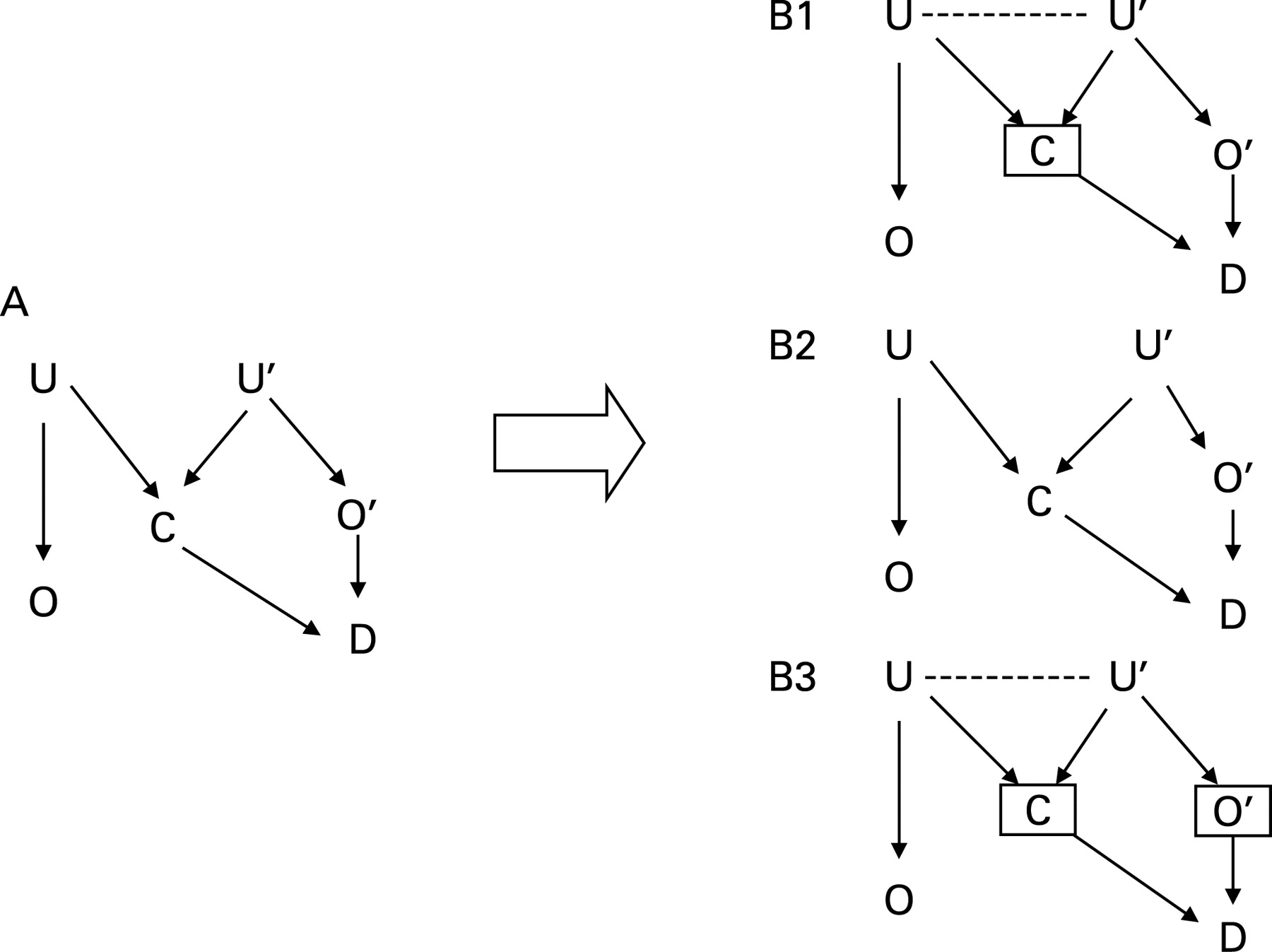
Contrary to what we have assumed in the scenarios 1 and 2, low SES is commonly associated with the risk of several cancer types.39 Let us therefore consider another scenario of a study investigating the association between having worked as a waiter (O) and lung cancer risk (D) (fig 3).

As for scenario 2, waiters tend to have a lower SES (C), which, in turn, is associated with having worked in occupations entailing exposure to known lung carcinogens (O′).40 However, in scenario 3, low SES (C) is also a determinant of lung cancer risk (D).39
This scenario is more complex than the previous two, because through the SES (C) there are two alternative paths connecting the occupational exposure of interest (O) with cancer risk (D) (fig 3A). As for scenario 2, the first path goes through the other occupational exposures (O′), so that SES (C) is a collider. However, SES (C) is a non-collider in the second path, because having worked as a waiter (O) is directly connected with the cancer risk (D) through SES (C). This implies that, on the one hand, the first path is opened and the second path is blocked after conditioning on SES (C) (fig 3B1), whereas, on the other hand, the first path is blocked and the second path is opened if SES (C) is not included in the model (fig 3B2). All paths are blocked when conditioning on SES (C) and other occupational exposures (O′) (fig 3B3). It follows that, if information on occupations entailing exposure to lung carcinogens is not available (O′), the crude estimate and the SES-adjusted estimate are biased, and the magnitude of the bias depends on the magnitude of the associations between the variables.
Data from a hypothetical study of employment as a waiter (O) and lung cancer risk (D) are summarized in table 2.
The prevalences of exposure to the occupation of interest (O) and to other occupations (O′), and the prevalences of subjects having low SES (C) are the same as for scenario 2 (table 1). It is moreover assumed that there is no (independent) association between having worked as a waiter and having worked in occupations entailing exposure to lung carcinogens (OROO′ = 1.0). Low SES (RRCD|O′ = 2.0) and having worked in occupations entailing exposure to lung carcinogens (RRO′D|C = 2.0) are associated with a twofold increased risk of lung cancer. The SES (C) and other occupations (O′) adjusted relative risk of lung cancer (D) for having worked as a waiter (O) is 1.0, whereas the crude estimate (RROD = 1.2) and the SES-adjusted estimate (RROD|C = 0.9) are biased.
Although we have assumed that SES (C) directly causes cancer (D), in practice there are several lifestyle factors that are intermediate between SES (C) and cancer (D), such as smoking, diet, physical exercise, etc. In studies of the association between working as a waiter (O) and lung cancer (D) risk, information on smoking and possibly diet is usually collected, and adjustment for these two intermediate factors could seem a reasonable alternative to adjustment for SES (C). However, being intermediate factors, smoking and diet are descendants of SES (C); hence, adjusting for these factors, similarly to the adjustment for SES (C) in fig 3B1, opens the path that connects the exposure of interest (O) with cancer risk (D) through other occupational exposures (O′). Moreover, there may be other lifestyle factors that are also intermediate between SES (C) and cancer (D), so adjusting for smoking and diet and other occupational exposures (O′) will still leave open the path that connects the exposure of interest (O) to the cancer risk (D) through SES (C).
Non-response bias
Participation in epidemiological studies may be associated with SES,41 and this may result in bias if participation is also related to the disease status. Under this circumstance participation (P) becomes a collider and is also a descendent of SES (C) (fig 4A).

Since analyses are always conducted among participants only, which ultimately means conditioning on participation (P), the path between SES (C) and cancer (D) risk is opened in this situation.32 This introduces a spurious association between SES (C) and cancer (D) risk (ie non-response bias), even when such an association is not present at the population level (fig 4B). Moreover, since participation (P) is a descendant of SES (C), conditioning on participation (P) ultimately introduces confounding through other occupational exposures (O′) (fig 4B). Therefore, adjustment for SES (C) would remove at least in part non-response bias, but confounding through other occupational exposures (O′) would remain.
DISCUSSION
In this paper, we have used DAGs to explore issues of adjustment for SES in occupational cancer studies. In some scenarios adjustment for SES makes no difference to the findings, in some it removes bias, and in some it introduces bias (unless there is also adjustment for other occupational exposures). These scenarios therefore illustrate the need for careful consideration of the relationship between variables before deciding on whether adjustment for SES is needed. Incorrect results may be obtained by the approach of simply adjusting for SES and including it in the model if it changes the estimate of the occupational status effect.
In developing and using such causal theories, it is also crucial to consider the nature of the association between SES and the occupational factor under study, since DAGs entirely depend on the assumptions about the causal relationships between the variables. According to counterfactual theory, an exposure causes an event in an individual (or population) if at least some cases of the event would not have occurred had the individual (or the population) remained unexposed.6 42 SES and occupational status meet this definition because, as noted in the third scenario in this paper, they belong to the causal pathway to the disease. We assumed that SES, especially adult SES (which is usually the measure of interest in occupational cancer studies) and occupational status share (unmeasured) common causes, such as the wealth and education of the family of origin. Conversely, if SES is assumed to be a cause of occupational status, our examples do not hold, whereas an indicator of SES could be always included in the model and will also control for other occupational exposures.43
The examples that we have discussed in this paper show that a unique answer to the issue of adjustment for SES in occupational cancer studies is not possible. As suggested above, in some instances this may be because SES and occupational factors are part of a complex social matrix and therefore cannot, and should not, be analysed separately.14 However, in many situations it is necessary to attempt to obtain a risk estimate specific for the occupational exposure while controlling for SES when this is appropriate. We have therefore derived some practical rules to decide on whether adjustment for SES is needed in such situations (fig 5).

These rules take into account (1) if SES is an indirect cause of the cancer under study; (2) the availability of information on other occupational factors; and (3) the relevance of the associations between, on the one hand, other occupational factors and cancer and, on the other hand, SES and the cancer under study. Although in some studies adjustment for SES is appropriate and in some it is not, when adult SES and other occupations are important risk factors for the cancer under study, we suggest that estimates adjusted for SES and crude estimates are reported so that the findings can be interpreted appropriately in the light of the possible causal models.
What is already known on this subject
There is debate on whether analyses of occupational cancer studies should be adjusted for SES, and no standard approach to deal with this issue has been established.
What this study adds
Adjustment for SES accommodates its possible confounding effect, but may also introduce bias if other occupational exposures cause the cancer under study.
A unique answer to the issue of adjustment for SES status in occupational cancer studies is not possible. If SES and other occupations are important risk factors for the cancer under study and no information on other occupational exposures is available, estimates adjusted for SES and crude estimates should be reported.
Policy implications
In future occupational cancer studies, decision about adjustment for SES should be based on the causal relationships between variables, rather than simply adjusting for SES and seeing if it makes a difference to the main effect estimates.
The decision about adjustment for SES should be clearly discussed and motivated in the manuscripts.
REFERENCES
Footnotes
Funding: This study has been conducted in the framework of projects supported by the Compagnia SanPaolo/FIRMS and the Italian Association for Research on Cancer (AIRC). Neil Pearce’s work on this paper was supported by the Health Research Council of New Zealand and the Progetto Lagrange, Fondazione CRT/ISI.
Competing interests: None.