


Abstract
The authors investigated the relation between ambient concentrations of five of the Environmental Protection Agency's criteria pollutants and asthma exacerbations (daily symptoms and use of rescue inhalers) among 990 children in eight North American cities during the 22-month prerandomization phase (November 1993–September 1995) of the Childhood Asthma Management Program. Short-term effects of carbon monoxide, nitrogen dioxide, particulate matter less than 10 μm in aerodynamic diameter (PM10), sulfur dioxide, and warm-season ozone were examined in both one-pollutant and two-pollutant models, using lags of up to 2 days. Lags in carbon monoxide and nitrogen dioxide were positively associated with both measures of asthma exacerbation, and the 3-day moving sum of sulfur dioxide levels was marginally related to asthma symptoms. PM10 and ozone were unrelated to exacerbations. The strongest effects tended to be seen with 2-day lags, where a 1-parts-per-million change in carbon monoxide and a 20-parts-per-billion change in nitrogen dioxide were associated with symptom odds ratios of 1.08 (95% confidence interval (CI): 1.02, 1.15) and 1.09 (95% CI: 1.03, 1.15), respectively, and with rate ratios for rescue inhaler use of 1.06 (95% CI: 1.01, 1.10) and 1.05 (95% CI: 1.01, 1.09), respectively. The authors believe that the observed carbon monoxide and nitrogen dioxide associations can probably be attributed to mobile-source emissions, though more research is required.
Many recent panel studies of the relation between air pollution concentrations and asthma aggravation in children have shown positive associations. Of the Environmental Protection Agency's six criteria pollutants, particulate matter and ozone have exhibited the most evidence of associations with asthma exacerbation (1–12). Still, carbon monoxide, nitrogen dioxide, and sulfur dioxide have also been linked to asthma aggravation (3, 5, 8, 10, 12). Because much of the evidence for a relation between air pollution and asthma aggravation has arisen from standard panel studies, which are carried out in a single geographic region and over a short time frame (e.g., a season), individual study results may not apply to different populations and longer periods of time. An analysis of 846 children participating in the National Cooperative Inner-City Asthma Study found that during the summer months, levels of ozone, nitrogen dioxide, and sulfur dioxide were associated with morning asthma symptoms in single-pollutant models (13), but particulate matter less than 10 μm in aerodynamic diameter (PM10) was not. In contrast to the smaller panel studies, the National Cooperative Inner-City Asthma Study examined these relations in children living in eight distinct cities, so its results may be more generally applicable.
We investigated the relation between daily ambient concentrations of carbon monoxide, nitrogen dioxide, ozone, PM10, and sulfur dioxide and daily asthma symptoms and rates of rescue inhaler use among 990 children in eight North American cities during the prerandomization phase of the Childhood Asthma Management Program (CAMP) (14). This report extends previous analyses of children who participated in CAMP at the Seattle, Washington, center (8, 12). In those analyses, Yu et al. (12) and Slaughter et al. (8) reported associations between carbon monoxide, PM10, and fine particulate matter (defined as <1 μm) and the risks of any asthma symptoms and more severe asthma symptoms, respectively. For example, a 1.11-fold increase (95 percent confidence interval (CI): 1.03, 1.20) in the odds of any symptoms (12) and a 1.10-fold increase (95 percent CI: 1.01, 1.18) in the odds of more severe symptoms (8) were observed per 10-μg/m3 difference in the 1-day lag of PM10.
The present report provides a unique contribution in that it can be considered a meta-analysis of eight large, within-city panel studies; however, it does not suffer from many of the challenges associated with meta-analyses in the published literature (e.g., between-study heterogeneity and obvious publication bias) (15). The large and geographically diverse panel of children participating in CAMP during the prerandomization phase was observed from November 1993 to September 1995, and individuals were followed for 1–6 months. This allowed us to examine the health effects of ambient concentrations of carbon monoxide, nitrogen dioxide, PM10, and sulfur dioxide across seasons and geographic regions. Because the health effects of ozone are thought to occur during the warm season, we limited the analysis of ozone to the months of May through September in 1994 and 1995. Like the findings from the National Cooperative Inner-City Asthma Study, results from this study may be applicable to a broad population, but with the exception of those pertaining to ozone, they are intended to represent year-round associations (e.g., averages of season-specific associations).
MATERIALS AND METHODS
CAMP is a National Heart, Lung, and Blood Institute-sponsored clinical trial that recruited children from eight North American cities: Albuquerque, New Mexico; Baltimore, Maryland; Boston, Massachusetts; Denver, Colorado; San Diego, California; Seattle, Washington; St. Louis, Missouri; and Toronto, Ontario, Canada. The primary purpose of CAMP is to evaluate the long-term effects of daily use of inhaled antiinflammatory medication on asthma status and lung growth in children with mild-to-moderate asthma (14). From the time when diary card completion began until randomization, children used albuterol as needed for symptoms and oral prednisone for exacerbations but were restricted from daily controller medication. At the end of each day, under the supervision of their families, the children completed daily diary cards to report their experience with asthma symptoms. The children and their families were carefully instructed on the importance of accurately reporting symptoms and medication use on the daily diary cards.
Inclusion criteria
All subjects studied here were randomized into the primary CAMP study, and inclusion criteria have been reported previously (14). Participants were excluded if we were able to verify that the centroid of the ZIP or postal code in which they lived was greater than 50 miles (80 km) from the nearest Aerometric Information Retrieval System pollutant monitor. Twelve children from Albuquerque, one from Baltimore, 16 from Denver, 10 from Seattle, four from St. Louis, and five from Toronto were excluded for this reason. Of the 1,041 children randomized into CAMP, 48 were excluded because of our 50-mile rule. Three additional children were excluded because information on a key measure of sensitivity, the methacholine concentration required to reduce forced expiratory volume in 1 second by 20 percent, was not available.
Ambient air pollution
Data on pollution concentrations were obtained from the Aerometric Information Retrieval System (www.epa.gov/air/data/index.html) for US cities and from Environment Canada (www.ec.gc.ca/envhome.html) for Toronto. Within each city, multiple monitors were used to measure ambient pollution concentrations. Monitor-specific concentrations were 24-hour averages for PM10, carbon monoxide, nitrogen dioxide, and sulfur dioxide and a 1-hour maximum for ozone. Daily, citywide concentrations were calculated by averaging monitor-specific concentrations, and an adjusted average was used on days on which only a fraction of monitors were in operation. Individual monitors that appeared to be recalibrated during the study (e.g., an obvious shift in pollution concentrations) were excluded from ambient pollution exposure calculations. For carbon monoxide, nitrogen dioxide, sulfur dioxide, and ozone, monitors that were in operation for at least half of the study days and, for PM10, monitors that were in operation for at least 90 of the study days were included in the ambient pollution exposure calculations.
The National Oceanic and Atmospheric Administration provided meteorologic data for the eight participating cities. Daily temperature and humidity measures were summarized using the maxima of hourly measurements. Wind speed was a 24-hour average, precipitation a daily sum, and stagnation a percentage of hourly measurements with wind speed measured below 6 miles/hour (9.6 km/hour).
Outcomes
Children recorded the severity of their asthma symptoms on daily diary cards completed at the end of each day. Asthma severity was coded as follows: 0 = no asthma symptoms; 1 = 1–3 mild asthma episodes, each lasting 2 hours or less; 2 = four or more mild asthma episodes or one or more episodes that temporarily interfered with activity, play, school, or sleep; and 3 = one or more asthma episodes lasting longer than 2 hours or resulting in shortening of normal activity, seeing a doctor for acute care, or going to a hospital for acute care. Daily diary cards on which symptom severity was not recorded (1.6 percent) were excluded from all analyses. Severity codes 1, 2, and 3 were collapsed into a single category to create a dichotomous response variable of any daily asthma symptoms versus none. On the diary cards, children also reported their daily number of rescue inhaler puffs. Since the standard dose of inhaled medication is two puffs, we defined one “use” of a rescue inhaler as half the standard number of puffs (i.e., one puff), and if an odd number of puffs was reported, we rounded up. The dichotomous variable of any asthma symptoms versus none and the number of rescue inhaler uses were the outcomes studied.
Statistical analysis
Models.
We sought to examine the relation between asthma aggravation and daily ambient air pollution concentrations for five criteria pollutants—carbon monoxide, nitrogen dioxide, ozone, PM10, and sulfur dioxide—across all cities. Towards this end, we constructed models within each city and then combined the city-specific parameter estimates to obtain the reported study-wide estimates using meta-analytic procedures (16). Since there is no general consensus regarding the appropriate day-lag of ambient concentrations to consider when studying their relations with asthma exacerbations, we examined the effects of 0-, 1-, and 2-day lags and the 3-day moving sum in separate models. The 3-day moving sum is the sum of the 0-, 1-, and 2-day lags in concentrations, and is therefore three times the 3-day moving average. One- and two-pollutant models were considered.
The generalized estimating equations procedure (17, 18) was used to estimate the marginal relation between asthma symptoms and rescue inhaler uses and ambient pollution concentrations in each city. Logistic and Poisson regression models were constructed for asthma symptoms and rescue inhaler uses, respectively. We report increases in the odds of asthma symptoms and in the rates of rescue inhaler use associated with large differences in exposure concentrations: carbon monoxide, 1.0 parts per million (ppm); nitrogen dioxide, 20 parts per billion (ppb); ozone, 30 ppb; PM10, 25 μg/m3; and sulfur dioxide, 10 ppb. For estimation, we used a working independence covariance structure, since multiple lags in exposure were potentially associated with both responses. In this setting, nonindependence covariance weighting can result in biased estimates (19, 20). Robust standard errors were used to account for the intraindividual correlations.
Daily ambient air pollution records were nearly complete for most pollutants, although data on sulfur dioxide in Albuquerque and data on nitrogen dioxide in Seattle were not collected and therefore were not included in our analyses. PM10 was measured on a daily basis in Seattle (97 percent of study days) and Albuquerque (99 percent of study days). In all other cities, it was measured regularly but only on a subset of days: 50 percent in Baltimore, 23 percent in Boston, 37 percent in Denver, 24 percent in San Diego, 19 percent in St. Louis, and 47 percent in Toronto. To recover a fraction of the missing PM10 data, we constructed 10 imputation data sets per city for analyses involving PM10. Meteorologic values (wind speed, stagnation, temperature, humidity), other pollutant concentrations, including 0- to 4-day lags, and daily summaries of asthma aggravation (e.g., the fraction of children experiencing asthma symptoms and the mean number of rescue inhaler uses) were used to impute missing PM10 values. Depending upon the city, the prediction models accounted for 50–75 percent of the variation in PM10 on days on which PM10 data were available. Within each city, regression analysis was done on each imputation data set, and results were combined to ascertain city-specific estimates using standard multiple imputation techniques (23).
Analysis approach.
We used SAS, version 8.02 (24), to manage all data and to build the multiple-imputation data sets. All regression modeling and the summarization of estimates was done with the R programming language (25), using the geepack (26), mitools (27), and rmeta (28) packages.
RESULTS
All subjects considered in this analysis were randomized into CAMP. A total of 990 children were studied (table 1). They were followed for a median of nearly 2 months and were 5–12 years old when diary card completion began (interquartile range, 7–10). Children reported asthma symptoms and rescue inhaler uses on 52 percent and 44 percent of all person-days, respectively, though in each city there were subjects who experienced symptoms or used the rescue inhaler on every day under study or on no days.
Characteristics of participants in the prerandomization phase of the Childhood Asthma Management Program, November 1993–September 1995
Albuquerque, New Mexico | Baltimore, Maryland | Boston, Massachusetts | Denver, Colorado | San Diego, California | Seattle, Washington | St. Louis, Missouri | Toronto, Ontario, Canada | All cities | |
|---|---|---|---|---|---|---|---|---|---|
| No. of children | 109 | 127 | 123 | 128 | 122 | 134 | 128 | 119 | 990 |
| No. of study days per child | |||||||||
| Median | 57 | 56 | 51 | 39 | 57 | 54 | 68 | 59 | 55 |
| IQR* | 46–74 | 48–70 | 43–64 | 33–44 | 49–77 | 47–67 | 55–79 | 48–74 | 44–70 |
| Range | 31–201 | 28–125 | 29–96 | 21–115 | 30–115 | 28–112 | 28–118 | 30–121 | 21–201 |
| Age (years) | |||||||||
| Median | 8.9 | 8.1 | 9.2 | 8.7 | 9.3 | 8.7 | 9.0 | 7.5 | 8.7 |
| IQR | 7.5–10.6 | 6.9–10.0 | 7.8–10.5 | 6.5–10.3 | 7.3–11.2 | 6.9–10.2 | 7.3–10.7 | 6.6–9.5 | 7.0–10.5 |
| Range | 5.1–12.7 | 5.0–12.8 | 5.0–12.8 | 5.0–12.9 | 5.0–<13.0 | 5.0–<13.0 | 5.0–<13.0 | 5.0–12.6 | 5.0–<13.0 |
| Sensitivity to the methacholine challenge (mg/ml)† | |||||||||
| Median | 1.047 | 0.905 | 1.094 | 1.751 | 0.924 | 0.691 | 1.570 | 1.139 | 1.095 |
| IQR | 0.326–2.866 | 0.499–2.140 | 0.518–3.002 | 1.007–4.377 | 0.444–1.894 | 0.322–1.727 | 0.657–4.164 | 0.617–2.635 | 0.501–2.703 |
| Range | 0.023–10.153 | 0.023–11.548 | 0.058–10.013 | 0.176–11.638 | 0.108–9.663 | 0.057–11.965 | 0.08–13.265 | 0.133–10.584 | 0.023–13.265 |
| Symptom score‡,§ | |||||||||
| 0 | 0.51 | 0.58 | 0.52 | 0.54 | 0.45 | 0.40 | 0.39 | 0.46 | 0.48 |
| 1 | 0.42 | 0.38 | 0.42 | 0.41 | 0.45 | 0.51 | 0.52 | 0.46 | 0.45 |
| 2 | 0.06 | 0.04 | 0.06 | 0.04 | 0.10 | 0.08 | 0.08 | 0.07 | 0.07 |
| 3 | 0.01 | 0.01 | 0.01 | 0.00 | 0.01 | 0.01 | 0.01 | 0.01 | 0.01 |
| Subject-specific proportion of days with symptom score >0¶ | |||||||||
| Median | 0.46 | 0.37 | 0.44 | 0.43 | 0.53 | 0.57 | 0.60 | 0.51 | 0.48 |
| IQR | 0.32–0.61 | 0.25–0.61 | 0.29–0.62 | 0.26–0.64 | 0.34–0.79 | 0.4–0.87 | 0.42–0.85 | 0.38–0.73 | 0.32–0.72 |
| Range | 0.07–1.00 | 0.00–1.00 | 0.00–1.00 | 0.00–1.00 | 0.04–1.00 | 0.03–1.00 | 0.15–1.00 | 0.04–1.00 | 0.00–1.00 |
| No. of rescue inhaler puffs per day‡ | |||||||||
| 0 | 0.56 | 0.60 | 0.70 | 0.57 | 0.54 | 0.44 | 0.47 | 0.60 | 0.56 |
| 1 | 0.37 | 0.36 | 0.25 | 0.38 | 0.37 | 0.45 | 0.41 | 0.33 | 0.37 |
| 2 | 0.05 | 0.03 | 0.04 | 0.05 | 0.08 | 0.10 | 0.10 | 0.06 | 0.07 |
| >2 | 0.01 | 0.00 | 0.01 | 0.00 | 0.01 | 0.01 | 0.02 | 0.01 | 0.01 |
| Subject-specific proportion of days with ≥1 rescue inhaler puff¶ | |||||||||
| Median | 0.40 | 0.34 | 0.23 | 0.40 | 0.44 | 0.55 | 0.48 | 0.36 | 0.40 |
| IQR | 0.24–0.59 | 0.20–0.54 | 0.09–0.42 | 0.19–0.65 | 0.25–0.67 | 0.33–0.81 | 0.33–0.78 | 0.20–0.56 | 0.22–0.65 |
| Range | 0.00–0.98 | 0.00–1.00 | 0.00–1.00 | 0.00–1.00 | 0.00–1.00 | 0.00–1.00 | 0.02–1.00 | 0.00–1.00 | 0.00–1.00 |
IQR, interquartile range.
The dose of methacholine required to decrease forced expiratory volume in 1 second by 20%.
Symptom score and rescue inhaler uses are given as the proportion of daily diary cards completed.
Symptom scores: 0 = no asthma symptoms; 1 = 1–3 mild asthma episodes, each lasting 2 hours or less; 2 = four or more mild asthma episodes or one or more episodes that temporarily interfered with activity, play, school, or sleep; and 3 = one or more asthma episodes lasting longer than 2 hours or resulting in shortening of normal activity, seeing a doctor for acute care, or going to a hospital for acute care.
In these calculations, a summary measure is represented for each subject (e.g., fraction of days with asthma symptom severity score X), and percentiles of the distribution of summary measures are reported.
Pollution concentrations during the study period are summarized in table 2. We report the number of monitors used in the calculations of daily ambient concentrations, percentiles of daily concentrations, and season-adjusted (partial) correlations among pollutants. Since PM10 data were recorded on a subset of study days in all cities except Seattle and Albuquerque, we summarized the distribution of PM10 values in each city with a single, complete imputation sample. All pollutants tended to be positively correlated with one another (note, however, that correlations with ozone correspond only to the months of May through September in 1994 and 1995). Carbon monoxide and nitrogen dioxide tended to be most highly correlated, with values ranging from 0.63 in Toronto to 0.92 in San Diego. Ozone tended to be less positively correlated with the other gases, though in several cities it was highly correlated with PM10.
Ambient air pollution concentrations and season-adjusted correlations in pollutants during the prerandomization phase of the Childhood Asthma Management Program, November 1993–September 1995*
City | No. of monitors† | Percentile‡ | Season-adjusted correlation§ | ||||||||||||||
|---|---|---|---|---|---|---|---|---|---|---|---|---|---|---|---|---|---|
| 10th | 25th | 50th | 75th | 90th | Nitrogen dioxide | Ozone | PM10 | Sulfur dioxide | |||||||||
| Albuquerque, New Mexico (November 25, 1993–August 29, 1995) | |||||||||||||||||
| Carbon monoxide (ppm¶ × 10) | 3 | 4.3 | 6.0 | 8.9 | 12.6 | 18.2 | 0.76 | 0.09 | 0.31 | ||||||||
| Nitrogen dioxide (ppb¶) | 1 | 9.8 | 12.8 | 17.8 | 25.1 | 34.3 | 1 | 0.04 | 0.26 | ||||||||
| Ozone (ppb) | 5 | 45.1 | 50.0 | 55.0 | 61.2 | 68.4 | 1 | 0.03 | |||||||||
| PM10 (μg/m3) | 2 | 11.5 | 15.5 | 20.6 | 27.0 | 33.5 | 1 | ||||||||||
| Sulfur dioxide (ppb) | 0 | ||||||||||||||||
| Baltimore, Maryland (November 9, 1993–August 13, 1995) | |||||||||||||||||
| Carbon monoxide (ppm × 10) | 6 | 4.1 | 5.6 | 7.3 | 9.9 | 14.9 | 0.69 | 0.21 | 0.51 | 0.50 | |||||||
| Nitrogen dioxide (ppb) | 2 | 16.5 | 20.8 | 25.8 | 31.5 | 36.9 | 1 | 0.44 | 0.62 | 0.49 | |||||||
| Ozone (ppb) | 13 | 41.4 | 52.1 | 65.8 | 82.7 | 94.7 | 1 | 0.73 | 0.30 | ||||||||
| PM10 (μg/m3) | 12 | 12.4 | 17.6 | 26.4 | 35.4 | 44.0 | 1 | 0.31 | |||||||||
| Sulfur dioxide (ppb) | 3 | 3.2 | 4.7 | 6.7 | 9.8 | 14.2 | |||||||||||
| Boston, Massachusetts (January 6, 1994–September 12, 1995) | |||||||||||||||||
| Carbon monoxide (ppm × 10) | 4 | 6.4 | 8.1 | 10.0 | 12.4 | 14.6 | 0.80 | 0.20 | 0.28 | 0.67 | |||||||
| Nitrogen dioxide (ppb) | 4 | 16.6 | 20.1 | 24.8 | 30.6 | 35.7 | 1 | 0.47 | 0.48 | 0.68 | |||||||
| Ozone (ppb) | 4 | 33.0 | 38.2 | 52.2 | 66.0 | 82.1 | 1 | 0.64 | 0.21 | ||||||||
| PM10 (μg/m3) | 5 | 9.8 | 14.5 | 20.4 | 26.2 | 32.5 | 1 | 0.36 | |||||||||
| Sulfur dioxide (ppb) | 5 | 2.7 | 3.7 | 5.8 | 9.1 | 14.1 | |||||||||||
| Denver, Colorado (November 3, 1993–June 15, 1995) | |||||||||||||||||
| Carbon monoxide (ppm × 10) | 7 | 5.1 | 6.3 | 8.1 | 12.5 | 18.8 | 0.85 | −0.28 | 0.66 | 0.53 | |||||||
| Nitrogen dioxide (ppb) | 4 | 14.9 | 19.0 | 23.3 | 28.6 | 34.6 | 1 | 0.24 | 0.64 | 0.56 | |||||||
| Ozone (ppb) | 8 | 40.2 | 51.7 | 60.5 | 67.9 | 73.0 | 1 | 0.49 | 0.22 | ||||||||
| PM10 (μg/m3) | 7 | 6.8 | 12.5 | 20.1 | 27.9 | 37.3 | 1 | 0.51 | |||||||||
| Sulfur dioxide (ppb) | 2 | 1.2 | 2.5 | 4.4 | 6.7 | 9.5 | |||||||||||
| San Diego, California (November 24, 1993–July 2, 1995) | |||||||||||||||||
| Carbon monoxide (ppm × 10) | 8 | 5.2 | 6.3 | 8.8 | 13.6 | 18.9 | 0.92 | 0.34 | 0.52 | 0.19 | |||||||
| Nitrogen dioxide (ppb) | 8 | 11.0 | 13.9 | 19.2 | 25.5 | 32.5 | 1 | 0.39 | 0.55 | 0.23 | |||||||
| Ozone (ppb) | 9 | 43.7 | 50.8 | 59.3 | 69.9 | 75.2 | 1 | 0.44 | −0.03 | ||||||||
| PM10 (μg/m3) | 7 | 13.7 | 22.4 | 32.4 | 42.7 | 53.9 | 1 | 0.32 | |||||||||
| Sulfur dioxide (ppb) | 3 | 1.2 | 1.7 | 2.2 | 3.1 | 4.4 | |||||||||||
| Seattle, Washington (November 3, 1993–August 15, 1995) | |||||||||||||||||
| Carbon monoxide (ppm × 10) | 8 | 10.1 | 12.3 | 14.9 | 19.0 | 24.0 | 0.34 | 0.88 | 0.62 | ||||||||
| Nitrogen dioxide (ppb) | 0 | 1 | |||||||||||||||
| Ozone (ppb) | 4 | 26.7 | 34.0 | 43.0 | 53.8 | 61.5 | 1 | 0.57 | 0.43 | ||||||||
| PM10 (μg/m3) | 4 | 11.4 | 15.2 | 22.0 | 30.2 | 44.0 | 1 | 0.65 | |||||||||
| Sulfur dioxide (ppb) | 4 | 3.7 | 4.7 | 6.0 | 7.5 | 9.5 | |||||||||||
| St. Louis, Missouri (November 12, 1993–August 21, 1995) | |||||||||||||||||
| Carbon monoxide (ppm × 10) | 6 | 4.6 | 5.4 | 6.3 | 7.7 | 9.5 | 0.71 | 0.44 | 0.24 | 0.34 | |||||||
| Nitrogen dioxide (ppb) | 8 | 11.5 | 14.5 | 18.3 | 22.4 | 26.7 | 1 | 0.42 | 0.45 | 0.58 | |||||||
| Ozone (ppb) | 13 | 38.5 | 48.3 | 59.3 | 73.4 | 86.4 | 1 | 0.69 | 0.33 | ||||||||
| PM10 (μg/m3) | 6 | 14.0 | 21.3 | 28.5 | 36.5 | 45.0 | 1 | 0.38 | |||||||||
| Sulfur dioxide (ppb) | 9 | 3.9 | 5.3 | 7.4 | 10.7 | 13.6 | |||||||||||
| Toronto, Ontario, Canada (December 10, 1993–July 25, 1995) | |||||||||||||||||
| Carbon monoxide (ppm × 10) | 4 | 5.7 | 8.0 | 9.7 | 11.3 | 12.7 | 0.63 | 0.16 | 0.37 | 0.55 | |||||||
| Nitrogen dioxide (ppb) | 4 | 17.5 | 21.3 | 26.0 | 31.5 | 37.0 | 1 | 0.40 | 0.64 | 0.63 | |||||||
| Ozone (ppb) | 4 | 27.5 | 33.6 | 43.5 | 56.5 | 67.1 | 1 | 0.70 | 0.44 | ||||||||
| PM10 (μg/m3) | 1 | 6.8 | 12.0 | 17.7 | 27.2 | 37.8 | 1 | 0.48 | |||||||||
| Sulfur dioxide (ppb) | 4 | 0.2 | 1.0 | 2.5 | 4.8 | 8.8 | |||||||||||
Data on concentrations of particulate matter less than 10 μm in aerodynamic diameter (PM10) were available for a subset of study days in Baltimore, Boston, Denver, San Diego, St. Louis, and Toronto. Percentiles and correlations with other pollutants were based on an imputation sample used in the primary analysis for PM10. Ozone values and correlations with other pollutants were limited to the warm season, which lasted from May through September in 1994 and 1995.
To be included in the calculation of daily ambient concentrations, monitors must have been functioning for at least half of the study days. Since PM10 was not measured daily in all cities, monitors were included in the calculation of daily ambient concentrations if they were functioning for at least 90 of the study days.
Daily, monitor-specific values were 24-hour averages for carbon monoxide, nitrogen dioxide, and sulfur dioxide and a 1-hour maximum for ozone. Daily, citywide ambient concentrations for all pollutants were calculated with an adjusted average over monitor-specific values.
Individual seasons used in the adjustments are given by consecutive 45-day time windows.
ppm, parts per million; ppb, parts per billion.
One-pollutant models
Study-wide estimates for asthma symptoms and rescue inhaler uses from one-pollutant models are displayed in figures 1 and 2, respectively. Lags in within-subject carbon monoxide and nitrogen dioxide concentrations showed the most evidence of a positive relation with both responses. The 3-day moving sum of sulfur dioxide was also positively associated with symptoms, but PM10 and warm-season ozone were not associated with exacerbations.
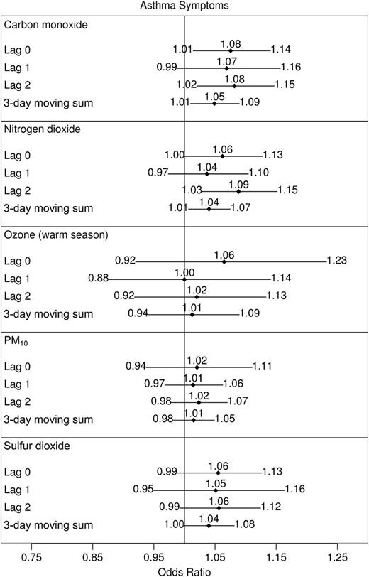
Odds ratios for daily asthma symptoms associated with shifts in within-subject concentrations of one air pollutant, Childhood Asthma Management Program, November 1993–September 1995. Effect sizes reported correspond to the following shifts: carbon monoxide, 1 part per million; nitrogen dioxide, 20 parts per billion (ppb); ozone, 30 ppb; particulate matter less than 10 μm in aerodynamic diameter (PM10), 25 μg/m3; and sulfur dioxide, 10 ppb. All city-specific estimates of pollutant effects were included in calculations of study-wide effects except sulfur dioxide in Albuquerque, New Mexico, and nitrogen dioxide in Seattle, Washington. Models corresponding to ozone were limited to the warm season (May through September in 1994 and 1995). Horizontal lines, 95% confidence interval (with limits specified at ends).
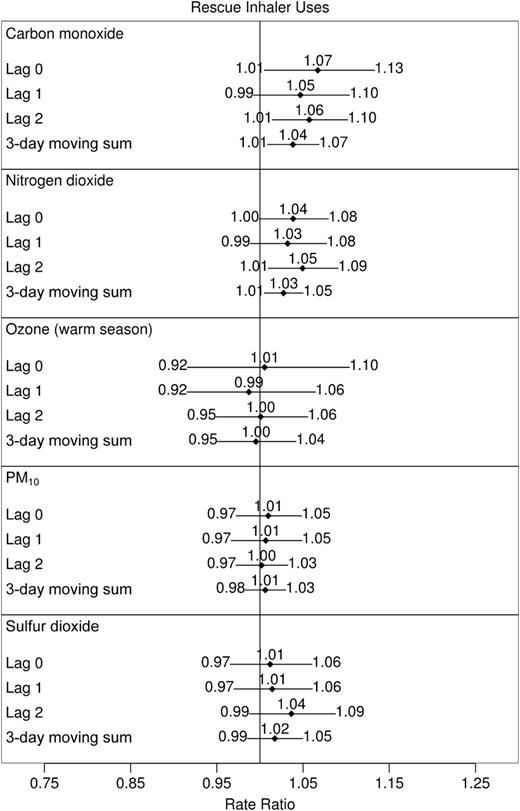
Rate ratios for number of rescue inhaler uses associated with shifts in within-subject concentrations of one air pollutant, Childhood Asthma Management Program, November 1993–September 1995. Effect sizes reported correspond to the following shifts: carbon monoxide, 1 part per million; nitrogen dioxide, 20 parts per billion (ppb); ozone, 30 ppb; particulate matter less than 10 μm in aerodynamic diameter (PM10), 25 μg/m3; and sulfur dioxide, 10 ppb. All city-specific estimates of pollutant effects were included in calculations of study-wide effects except sulfur dioxide in Albuquerque, New Mexico, and nitrogen dioxide in Seattle, Washington. Models corresponding to ozone were limited to the warm season (May through September in 1994 and 1995). Horizontal lines, 95% confidence interval (with limits specified at ends).
One-ppm differences in within-subject carbon monoxide concentrations were associated with symptom odds ratios of 1.08 (95 percent CI: 1.01, 1.14), 1.07 (95 percent CI: 0.99, 1.16), 1.08 (95 percent CI: 1.02, 1.15), and 1.05 (95 percent CI: 1.01, 1.09) for the 0-, 1-, and 2-day lags and the 3-day moving sum, respectively. Odds ratios associated with 20-ppb differences in nitrogen dioxide were 1.06 (95 percent CI: 1.00, 1.13), 1.04 (95 percent CI: 0.97, 1.10), 1.09 (95 percent CI: 1.03, 1.15), and 1.04 (95 percent CI: 1.01, 1.07), respectively. Although sulfur dioxide lags were positively related to risk of asthma symptoms, only the 3-day moving sum effect would be considered (marginally) statistically significant at the 0.05 level. A 1-ppb change in the 3-day moving sum of sulfur dioxide levels led to a 1.04-fold increase in the odds of symptoms (95 percent CI: 1.00, 1.08).
The results from single-pollutant models of rescue inhaler use were consistent with those of asthma symptoms. Relative rates of rescue inhaler use associated with a 1-ppm change in 0-, 1- and 2- day lags of carbon monoxide and the 3-day moving sum of carbon monoxide were 1.07 (95 percent CI: 1.01, 1.13), 1.05 (95 percent CI: 0.99, 1.10), 1.06 (95 percent CI: 1.01, 1.10), and 1.04 (95 percent CI: 1.01, 1.07), respectively, while 20-ppb shifts in the 0-, 1-, and 2-day lags of nitrogen dioxide and the 3-day moving sum of nitrogen dioxide led to relative rates of rescue inhaler use of 1.04 (95 percent CI: 1.00, 1.08), 1.03 (95 percent CI: 0.99, 1.08), 1.05 (95 percent CI: 1.01, 1.09), and 1.03 (95 percent CI: 1.01, 1.05), respectively. Sulfur dioxide was not associated with rescue inhaler use rates.
Two-pollutant models
Results from two-pollutant models were based on the sum of the two within-subject pollutant effects, as described in the “Analysis approach” section. Thus, they are intended to provide insight into the increased risk of asthma exacerbation associated with (simultaneous) shifts in two pollutants. As with the one-pollutant models, effects are characterized by increases in the odds of asthma symptoms and the rates of rescue inhaler use.
The effects of shifts in pairs of carbon monoxide, nitrogen dioxide, PM10, and sulfur dioxide levels on asthma symptoms and rescue inhaler uses are displayed in figures 3 and 4, respectively. Ozone was not included in two-pollutant models, since it is a warm-season pollutant, and our primary goal was to study year-round effects. While all lags in the pairs of pollutants exhibited positive relations with both responses, simultaneous shifts in 2-day lags of pairs of pollutants tended to have the largest impact on asthma aggravation. Among combinations of carbon monoxide, nitrogen dioxide, PM10, and sulfur dioxide, the 2-day lags in all models involving either carbon monoxide or nitrogen dioxide were associated with both responses, with 95 percent confidence intervals excluding 1. Simultaneous standardized shifts in the 2-day lags of these two pollutants led to a 1.09-fold increase in the odds of asthma symptoms (95 percent CI: 1.02, 1.16) and a 1.07-fold increase in the daily rate of rescue inhaler uses (95 percent CI: 1.02, 1.12). Simultaneous shifts in 3-day moving sums of two pollutants were also frequently (marginally) related to exacerbations.
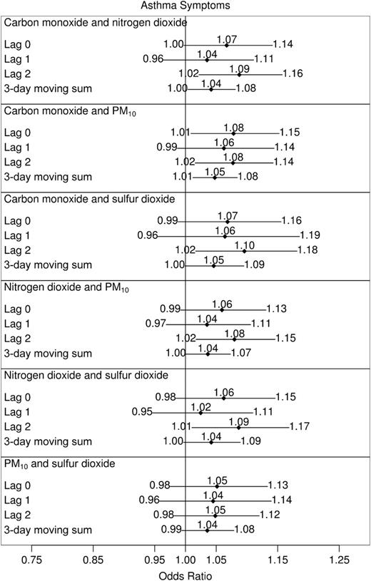
Odds ratios for daily asthma symptoms associated with shifts in within-subject concentrations of two air pollutants, Childhood Asthma Management Program, November 1993–September 1995. Effect sizes reported correspond to the following shifts: carbon monoxide, 1 part per million; nitrogen dioxide, 20 parts per billion (ppb); particulate matter less than 10 μm in aerodynamic diameter (PM10), 25 μg/m3; and sulfur dioxide, 10 ppb. All city-specific estimates of pollutant effects were included in calculations of study-wide effects except sulfur dioxide in Albuquerque, New Mexico, and nitrogen dioxide in Seattle, Washington. Horizontal lines, 95% confidence interval (with limits specified at ends).
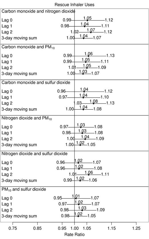
Rate ratios for number of rescue inhaler uses associated with shifts in within-subject concentrations of two air pollutants, Childhood Asthma Management Program, November 1993–September 1995. Effect sizes reported correspond to the following shifts: carbon monoxide, 1 part per million; nitrogen dioxide, 20 parts per billion (ppb); particulate matter less than 10 μm in aerodynamic diameter (PM10), 25 μg/m3; and sulfur dioxide, 10 ppb. All city-specific estimates of pollutant effects were included in calculations of study-wide effects except sulfur dioxide in Albuquerque, New Mexico, and nitrogen dioxide in Seattle, Washington. Horizontal lines, 95% confidence interval (with limits specified at ends).
Although the relation between the responses and the 0- and 1-day lags in ambient concentrations did not appear to be as strong as the 2-day lags, they were consistent with them (e.g., estimated odds ratios for symptoms and rate ratios for inhaler uses were greater than 1). The strongest among the 0- and 1-day lagged effects was observed with asthma symptoms: Shifts in the 0-day lag of carbon monoxide and PM10 resulted in an odds ratio of 1.08 (95 percent CI: 1.01, 1.15).
DISCUSSION
The goal of this panel-study analysis was to describe the relations between ambient concentrations of five of the Environmental Protection Agency's criteria pollutants and asthma exacerbation in children with mild-to-moderate asthma. Two important features of this study are that children lived in cities widely separated across North America and the entire observation period covered approximately 22 months. Thus, results reflect ambient air pollution effects averaged across seasons and geographic regions. Most previous panel studies of this subject examined these relations within a season and/or geographic region (1–12). Although the relations we estimated are implicitly different from those reported in previous research, acknowledging the large exposure differences used to characterize effect size, the observed associations were generally smaller than those from previous reports.
Among the pollutants studied, carbon monoxide and nitrogen dioxide appeared to capture the most relevant health information. Sulfur dioxide showed less evidence for a relation with asthma exacerbations unless it was considered in combination with carbon monoxide or nitrogen dioxide. There was no evidence of a warm-season effect of ozone or of a year-round effect of PM10. Mobile-source emissions contribute directly to concentrations of ambient carbon monoxide, nitrogen dioxide, and particulate matter (especially the fine fraction of PM10) and secondarily to ozone concentrations. In the cities we studied, carbon monoxide and nitrogen dioxide were highly correlated with one another, which is consistent with mobile emissions being a primary source of these pollutants. Carbon monoxide can interfere with oxygen transport through the formation of carboxyhemoglobin, and nitrogen dioxide has been shown to sensitize reactions to inhaled allergens (29–31); however, the observed association between carbon monoxide and nitrogen dioxide and risk of symptoms and rescue inhaler use should perhaps be interpreted with caution. Correlates of carbon monoxide and nitrogen dioxide emanating from mobile sources, including the fine fraction of PM10, which was not measured explicitly in the majority of our study cities, have also been shown to be associated with asthma exacerbation in children (3, 7, 8, 12). Another report suggested that ambient carbon monoxide, and perhaps nitrogen dioxide in the winter, could serve as a surrogate measure for the fine fraction of ambient PM10 (32). We believe carbon monoxide and nitrogen dioxide effects are more likely the effects of other pollutants emanating from mobile sources. Air stagnation can, in certain circumstances, be a reasonable surrogate for fine particulate matter (33, 34). To evaluate the hypothesis that the carbon monoxide and nitrogen dioxide effects were driven by mobile-source emissions, we replicated the one-pollutant analyses using number of stagnant hours per day as the predictor of interest. Although all lags of stagnation showed positive associations with exacerbations, none were statistically significant at the 0.05 level.
In contrast to several past studies (1–12), ambient PM10 and warm-season ozone concentrations were unrelated to exacerbations. PM10 concentrations were measured on less than 50 percent of study days in all cities except Seattle and Albuquerque. Thus, referring to it as PM10 may be may be misleading, and perhaps “estimated PM10” would be more appropriate. Imputation techniques can be used to recover a fraction of missing data; however, we acknowledge that there was a significant amount of missing information that was not recovered. In single-pollutant models, the estimated relative increase in variance due to missing PM10 data in cities other than Seattle and Albuquerque ranged from 10 percent to 24 percent for asthma symptoms and from 5 percent to 33 percent for rescue inhaler uses. Attenuation of parameter estimates was also possible because of the error associated with imputing PM10 concentrations using other pollutants, meteorologic variables, and daily summaries of children's asthma experiences. In the presence of other pollutant concentrations and meteorologic variables, daily summaries of individual responses were not informative, and our choice to include them when constructing imputation data sets had no impact on our conclusions. While PM10 effects were not observed for the entire panel of children, they were observed in recent reports on the children participating at the Seattle center (8, 12).
While the lack of observed association between ozone and exacerbations during the warm season was not expected, the strength of this study was in the total number of children observed and in the length of the observation period. A total of 990 children were followed over the course of 22 months; however, on a given day, the average number of children observed was approximately 12 per city, making season-specific effects difficult to capture. More thorough city-specific analyses may also be appropriate for the analysis of ozone.
Although year-round follow-up of children made this study unique and allowed us to address novel questions, relative to many panel studies, it was more susceptible to seasonal confounding. We constructed regression models with this concern in mind and took care to adjust for seasonal factors. We also conducted sensitivity analyses, examining more flexible seasonal confounding control (e.g., more seasons), which led to similar qualitative conclusions. Nevertheless, we must acknowledge that seasonal confounding may persist.
The National Center for Health Statistics estimated that, in 2003, 12 percent of children under age 18 years had ever been diagnosed with asthma and 6 percent had had an asthma attack in the past 12 months (35). In another study, children aged 13–14 years from three US study sites (in two cities) reported wheezing in the past 12 months and ever having asthma at rates of 20 percent and 17 percent, respectively (36, 37). In 1996, an estimated 2.5 million US children sought health care for asthma (38) and 6.3 million school absence days were attributed to asthma (38), and in 1998, the cost of asthma in the United States was estimated to be $12.8 billion per year (39). While asthma prevalence had been on the rise over the past several decades (40), this trend appears to have plateaued in recent years (41). We observed year-round associations between ambient concentrations of carbon monoxide and nitrogen dioxide and asthma exacerbations which we believe may represent mobile-source emission (fine particulate matter) effects. Though these relations are modest, they are clinically relevant, considering the enormous burden asthma places on the population at large. Further investigation is required, however, to explore the potential surrogacy of carbon monoxide and nitrogen dioxide for mobile-source emissions.
This research was partially funded by Environmental Protection Agency grant R827355. The Childhood Asthma Management Program is supported by contracts N01-HR-16044, -16045, -16046, -16047, -16048, -16049, -16050, -16051, and -16052 with the National Heart, Lung, and Blood Institute.
A portion of Dr. Jonathan Schildcrout's salary is funded by Pfizer Inc. (New York, New York).
References
Delfino RJ, Coate BD, Zeiger RS, et al. Daily asthma severity in relation to personal ozone exposure and outdoor fungal spores.
Delfino RJ, Zeiger RS, Seltzer JM, et al. Symptoms in pediatric asthmatics and air pollution: differences in effects by symptom severity, anti-inflammatory medication use and particulate averaging time.
Ostro B, Lipsett M, Mann J, et al. Air pollution and exacerbation of asthma in African-American children in Los Angeles.
Ostro B, Lipsett MJ, Mann JK, et al. Air pollution and asthma exacerbation among African-American children in Los Angeles.
Peters A, Goldstein IF, Beyer U, et al. Acute health effects of exposure to high levels of air pollution in Eastern Europe.
Romieu I, Meneses F, Ruiz S, et al. Effects of intermittent ozone exposure on peak expiratory flow and respiratory symptoms among asthmatic children in Mexico City.
Romieu I, Meneses F, Ruiz S, et al. Effects of air pollution on the respiratory health of asthmatic children living in Mexico City.
Slaughter JC, Lumley T, Sheppard L, et al. Effects of ambient air pollution on symptom severity and medication use in children with asthma.
Thurston GD, Lippmann M, Scott MB, et al. Summertime haze air pollution and children with asthma.
Timonen KL, Pekkanen J. Air pollution and respiratory health among children with asthmatic or cough symptoms.
Vedal S, Petkau J, White R, et al. Acute effects of ambient inhalable particles in asthmatic and nonasthmatic children.
Yu O, Sheppard L, Lumley T, et al. Effects of ambient air pollution on symptoms of asthma in Seattle-area children enrolled in the CAMP study.
Mortimer KM, Neas LM, Dockery DW, et al. The effect of air pollution on inner-city children with asthma.
Long-term effects of budesonide or nedocromil in children with asthma. The Childhood Asthma Management Program Research Group.
Ward DJ, Ayres JG. Particulate air pollution and panel studies in children: a systematic review.
Liang KY, Zeger SL. Longitudinal data analysis using generalized linear models.
Zeger SL, Liang KY. Longitudinal data analysis for discrete and continuous outcomes.
Pepe MS, Anderson GI. A cautionary note on inference for marginal regression models with longitudinal data and general correlated response data.
Schildcrout JS, Heagerty PJ. Regression analysis of longitudinal binary data with time-dependent environmental covariates: bias and efficiency.
Sheppard L. Insights on bias and information in group-level studies.
Neuhaus JM, Kalbfleisch JD. Between- and within-cluster covariate effects in the analysis of clustered data.
Rubin DB. Multiple imputation for nonresponse in surveys. New York, NY: John Wiley & Sons, Inc,
R Development Core Team. R: a language and environment for statistical computing. Vienna, Austria: R Foundation for Statistical Computing,
Lumley T. mitools: tools for multiple imputation of missing data. (R package, version 1.0). Vienna, Austria: R Foundation for Statistical Computing,
Lumley T. rmeta: meta-analysis. (R package, version 2.12). Vienna, Austria: R Foundation for Statistical Computing,
Bernstein JA, Alexis N, Barnes C, et al. Health effects of air pollution.
Strand V, Rak S, Svartengren M, et al. Nitrogen dioxide exposure enhances asthmatic reaction to inhaled allergen in subjects with asthma.
Tunnicliffe WS, Burge PS, Ayres JG. Effect of domestic concentrations of nitrogen dioxide on airway responses to inhaled allergen in asthmatic patients.
Sarnat JA, Brown KW, Schwartz J, et al. Ambient gas concentrations and personal particulate matter exposures: implications for studying the health effects of particles.
Norris G, Larson T, Koenig J, et al. Asthma aggravation, combustion, and stagnant air.
Slaughter JC, Kim E, Sheppard L, et al. Association between particulate matter and emergency room visits, hospital admissions and mortality in Spokane, Washington.
Dey AN, Bloom B. Summary health statistics for U.S. children: National Health Interview Survey,
Worldwide variations in the prevalence of asthma symptoms: The International Study of Asthma and Allergies in Childhood (ISAAC).
Worldwide variation in prevalence of symptoms of asthma, allergic rhinoconjunctivitis, and atopic eczema: ISAAC. The International Study of Asthma and Allergies in Childhood (ISAAC) Steering Committee.
Wang LY, Zhong Y, Wheeler L. Direct and indirect costs of asthma in school-age children.
Weiss KB, Sullivan SD. The health economics of asthma and rhinitis. I. Assessing the economic impact.
Beasley R. The burden of asthma with specific reference to the United States.

