Article Text

Statistics from Altmetric.com
In 1929 von Neergaard demonstrated that surface forces are responsible for a large part of the elastic recoil pressure of the lungs.1 This was evidenced by recordings of elastic recoil during deflation of air- and liquid-filled lungs. On the basis of similar experiments, extended to include inflation (fig 1), Radford laid down concepts which still form the basis for the interpretation of elastic pressure–volume (Pel–V) curves in today’s intensive care units.2 In this review these concepts will be analysed. The relevance of Pel–V curves as guidelines in managing ventilation to avoid lung trauma will be discussed. Furthermore, techniques for recording and analysis of Pel–V curves will be briefly commented upon.
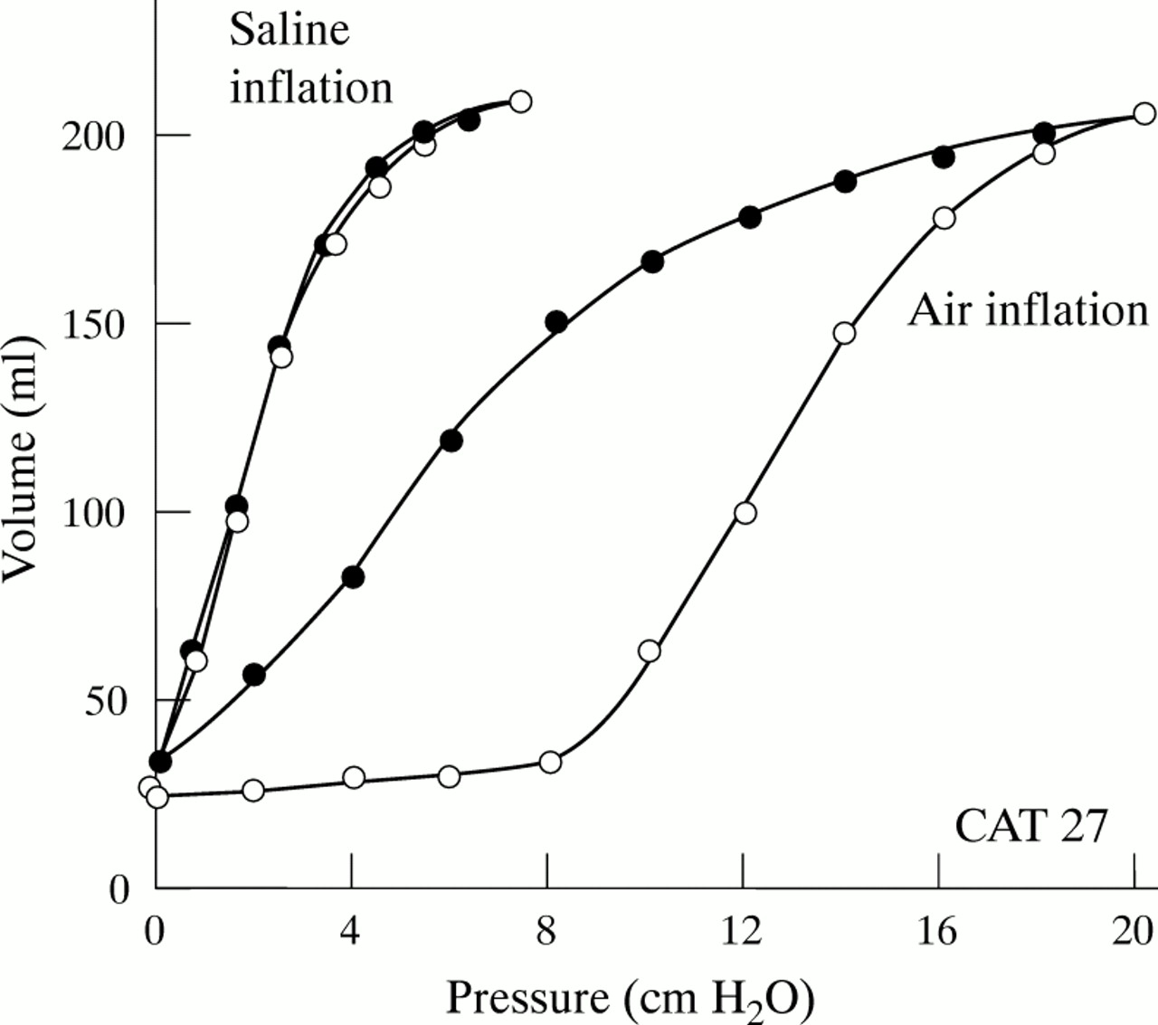
Pulmonary pressure–volume curves obtained during inflation and deflation with air and saline.2 The higher elastic recoil pressure during air deflation shows that surface tension contributes to lung recoil. It can be seen that during inflation with air a lower inflection point is followed by a steep, nearly linear, segment.
Features of the elastic pressure–volume curve
Pel–V curves are often recorded during an insufflation of gas which is preceded by an expiration to the elastic equilibrium volume. An example of an inspiratory Pel–V curve recorded from a patient with acute lung injury (ALI) is shown in fig 2. The features of the curve are well known.3 ,4 The curve can be considered to consist of three segments: an initial flat segment reflects a very low compliance, indicating collapse of peripheral airways and/or lung units preventing lung inflation; there then follows a segment with a steeper slope (that is, greater compliance); the transition between these two segments, which may be more or less abrupt, can be denoted the lower inflection point (LIP). Compliance remains stable over the second “linear” segment, as shown in various species.4-7 At large volumes and high pressures the slope—that is, the compliance—decreases. In fact, the compliance approaches zero when the respiratory system is extensively distended.7-10 The point at which a decrease in compliance is identified can be denoted the upper inflection point (UIP). The segment between the LIP and the UIP represents a zone of optimal compliance over which tidal ventilation should preferentially occur in order to protect the lung from trauma. However, this interpretation of the Pel–V curve should be critically analysed. To this end, we investigated a multi-compartment lung model.

The elastic pressure–volume (Pel–V) curve recorded over an extended volume range from a patient with acute lung injury. The smooth curve is calculated according to a three segment model. The dotted line represents the extrapolation of the linear segment of the Pel–V curve.
Multi-compartment lung model
The lung model comprises 100 units with a distribution of properties. The variations in properties are intended to mimic the non-homogeneity of the opening pressure of collapsed lung units as observed in ALI and in the acute respiratory distress syndrome (ARDS) by, for example, Gattinoni et al. 11 The units are subjected to different distending pressures corresponding to the pleural pressure gradient which is increased in ALI/ARDS due to the increase in lung density. The increased density will attenuate the distending pressure of lower lung units.
When the lung model is assumed to be fully recruited, it has a compliance of 50 ml/cm H2O which is constant up to a Pel of 14 cm H2O. At higher pressures the compliance falls and approaches zero at a fictive maximum volume of 1500 ml. The “ideal” Pel–V curve representing the fully recruited lung is shown in fig 3.
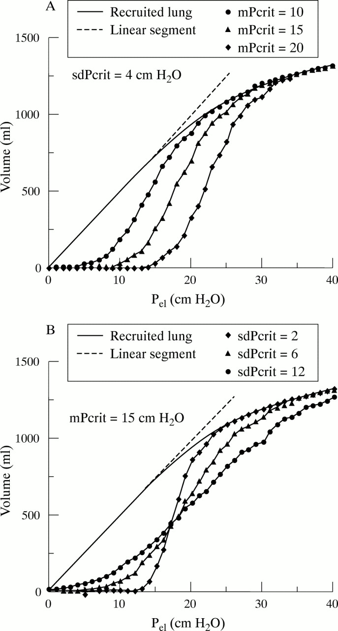
(A) Elastic pressure–volume (Pel–V) curves representing a multi-compartment lung model. The continuous curve shows features of a completely recruited lung. The other curves represent three lungs with mean critical opening pressures (mPcrit) of 10–20 cm H2O and a standard deviation of mPcrit (sdPcrit) of 4 cm H2O. (B) Three lungs with similar mPcrit (15 cm H2O) and an sdPcrit varying from 2 to 12 cm H2O.
Each of the 100 lung units has an identical Pel–V curve if the unit is recruited. For simplicity it was assumed that a lung unit would collapse or be recruited from the collapsed state at a specific critical pressure in the proximal airway (Pcrit). The distribution of the critical pressure between the lung units is defined by three parameters: the mean critical pressure (mPcrit), the standard deviation of Pcrit (sdPcrit), and the contribution to the surrounding pressure caused by lung weight, defined by the lung density and the vertical position of the unit. During insufflation a lung unit is considered to “pop” open when the airway pressure reaches the specific value of Pcrit for the unit. When the unit pops open the volume increases from zero to the volume of other open units. At higher airway pressure it is distended in accordance with the Pel–V curve of open units. This simple model does not include any resistive or viscoelastic properties.
When mPcrit is allowed to vary between 10 and 20 cm H2O at a constant sdPcrit of 4 cm H2O, an LIP is observed at a pressure slightly lower than mPcrit (fig 3A). Above the LIP a nearly linear segment shows a compliance which is far higher than the compliance of the fully recruited lung at similar pressures. The UIP is strongly dependent on the mPcrit and can be identified at a pressure of about 17–27 cm H2O. Full recruitment occurs at a much higher pressure, as indicated by the coalescence of Pel–V curves with the curve representing the fully recruited lung.
In order to simulate an augmented non-homogeneity of the lung with respect to the critical opening pressure, the sdPcrit was increased from 2 to 12 cm H2O while the mPcrit was kept constant at 15 cm H2O. The LIP is then observed at a lower pressure, the UIP at a higher pressure, and the compliance is lower (fig 3B).
Differences in the pleural pressure gradient were simulated by varying the lung density between 0.2 and 0.8 g/ml while keeping the values of mPcrit and sdPcrit constant. Higher densities led to a shift of the Pel–V curve towards higher pressures. Accordingly, the pleural pressure gradient affects the determination of the LIP and the UIP. The compliance of the linear segment decreased slightly at a higher lung density.
Significance of compliance
The results of these simulations merit some discussion of the significance of compliance. Compliance is defined as the volume change divided by the pressure change: C = ΔV/ΔP (Eqn 1) where ΔV consists of two components: ΔVdist represents the continuous distension of open lung units under increasing pressure, while ΔVrecr represents the volume increments when the critical opening pressure of one or more collapsed lung units is overcome and the units are recruited. Thus: C = ΔV/ΔP = (ΔVdist + ΔVrecr)/ΔP (Eqn 2)
For a given lung unit ΔVrecr is a sudden event when the unit “pops open”. For the whole lung ΔVrecr may appear as a continuous process when more and more lung units open up. Returning to the model experiments, a rather abrupt increase in compliance, identified as an LIP, indicates the commencement of recruitment of lung units. The subsequent, almost linear, segment with a high compliance reflects distension and recruitment occurring in parallel. A relatively homogeneous opening pressure of collapsed lung units causes a particularly high maximum compliance. The UIP indicates the end of significant recruitment. These implications of the model experiment deviate from the commonly held paradigm of the Pel–V curve, according to which the linear segment of the Pel–V curve represents a zone of optimal distensibility within which the tidal ventilation should occur in order to avoid lung collapse below the LIP and lung overdistension above the UIP.
The question arises: is the multi-compartment model realistic enough to merit a new view of the Pel–V curve? The model assumes that the Pel–V curve of recruited lung units and the total recruited lung is characterised by a linear segment followed by a segment with falling compliance. This assumption is fairly well supported by common knowledge. The absence of resistive and viscoelastic properties implies limitations in the model. However, such properties are also non-homogeneous and would tend to increase the spread in the values of time, pressure, and volume at which lung units are recruited during lung inflation. A model incorporating these properties would be more realistic. Such a model would lead to even more serious deviations from the concept that the linear segment represents the zone within which collapse/recruitment and overdistension are avoided.
The concept that the recruitment process in itself leads to a high value of compliance measured from the slope of the Pel–V curves is, indeed, indicated by the recordings of Radford (fig1).2 During inflation with air an LIP is observed at about 8 cm H2O. It is followed by a long, nearly linear, segment with a steep slope signifying a high compliance. At corresponding pressures the value of compliance is much lower during the succeeding deflation. The particularly high compliance over a large segment following the LIP during insufflation can be explained by continuing recruitment, which corresponds to contributions from ΔVrecr in equation 2.
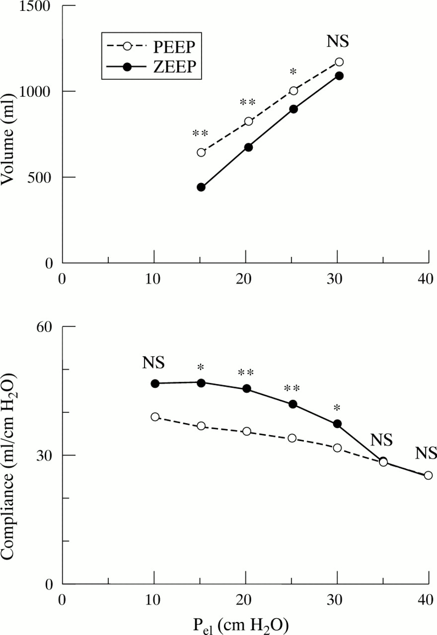
In a recent study12 it was reported that, in healthy anaesthetised humans, Pel–V curves recorded before and after a manoeuvre serving to recruit the lung13 showed quite different characteristics (fig 4). Before the recruitment manoeuvre an LIP was observed at about 20 cm H2O. Above the LIP a linear segment extending up to the maximum pressure of about 30 cm H2O was often observed. After the manoeuvre the LIP was observed at a pressure of about 13 cm H2O and the linear segment ceased at a UIP of only about 19 cm H2O. The compliance calculated from the uppermost part of the Pel–V curve was higher before the recruitment manoeuvre than after it. The conclusion was drawn that the high compliance above the LIP up to high volumes and pressures before the recruitment manoeuvre could be explained by ongoing recruitment. In ALI and ARDS it has been reported that Pel–V curves recorded after a single expiration to zero end-expiratory pressure showed a steeper slope (greater compliance) than curves recorded after expiration to a positive end-expiratory pressure (fig 5).14 It was concluded that the recruitment was a process which started at the LIP and which continued above the LIP over a large and steep segment of the Pel–V curve. Thus, accumulating experimental data show that the process of recruitment leads to a higher value of compliance as is suggested in equation 2.


Mean volume and compliance versus elastic pressure (Pel ) in 11 patients with ALI/ARDS. The recording was started after either an expiration to zero end expiratory pressure (ZEEP) or after an expiration at the clinically applied positive end expiratory pressure (PEEP). NS = non-significant; *p<0.05, **p<0.01. Modified from reference 14.
When in the operating theatre a collapsed lung is re-expanded, one may observe how lung units start to pop open at modest insufflation pressures. Complete lung recruitment occurs when the open areas coalesce at high distending pressures. Even in health, high airway pressures are required to re-inflate condensed lung zones.13 Recent observations by Gattinoniet al show that in ARDS recruitment occurs over a wide range of airway pressure.11 Therefore, a model with a wide distribution of opening pressures is realistic. Present knowledge thus supports the hypothesis that inhomogeneity between lung compartments may affect the Pel–V curve significantly, as indicated in fig 3B.
The Pel–V curve represents the integral over the curves from all lung units. The density of information in the Pel–V curves makes their interpretation difficult. As recent studies have shown, recordings repeated under different conditions may help us to interpret Pel–V curves better.10 ,14 Techniques allowing studies under strictly controlled conditions are thus necessary.
Recording of Pel–V curves in intensive care
STATIC Pel–V CURVES
Studies of the purely elastic properties of the respiratory system rely upon the determination of static elastic Pel–V curves. Most of our present knowledge on the static elastic relationship has been acquired with the super syringe method.3 ,15 Continuous gas exchange during the measurements and other practical problems16 ,17 have motivated the successive development of the flow interruption method.18-22 Recently, the introduction of computer control for a commercial ventilator (ServoVentilator 900C, Siemens-Elema AB, Sweden) offered the possibility of precise control of events preceding and during measurements of the static Pel–V relationship.23 The flow and pressure transducers of the ventilator were used. An even distribution of data along the curve and the elimination of heart synchronous artefacts are features which contribute to high precision and reproducibility. With the flow interruption method each of about 20 interrupted breaths is followed by a pause of some seconds. The interrupted breaths must be separated by at least two ordinary breaths. Thus, even when automated, the recording of the static Pel–V curve takes some minutes to perform.
When the ultimate goal of Pel–V curve recording is to avoid lung trauma during mechanical ventilation, one may ask whether the static elastic recoil pressure is the most relevant pressure to measure. Indeed, static pressures exist only under the artificial pauses used for its determination. During inspiration the dynamic pressure in the peripheral lung units is the sum of the static elastic and the viscoelastic recoil pressure. It seems unlikely that the viscoelastic pressure component of the dynamic pressure would induce less trauma than a corresponding static elastic pressure. Dynamic pressure recordings may then be more relevant with regard to the goal of the measurement. Such considerations, in combination with the practical problems associated with the determination of the static Pel–V curve, have motivated the search for alternative methods.
DYNAMIC Pel–V CURVES
Suratt and Owens24 and Ranieri et al 25 applied the concept that, at constant flow insufflation, variations in the rate of pressure change indicate a change in compliance. To minimise the resistive pressure Mankikianet al used a very low constant inspiratory flow.26 The flow rate was so low that continuous gas exchange caused artefacts similar to those in the super syringe technique. Servillo et al employed the above mentioned computer controlled ventilator for dynamic studies.27 After an expiration, with a duration and an end expiratory airway pressure defined by the user, a selected volume was delivered during a prolonged insufflation. The resistive pressure down to the trachea was subtracted. (The tube resistance was determined in vitro.) The airway resistance was measured during an ordinary breath and was used to subtract the airway resistive pressure. In ALI and ARDS the dynamic Pel–V curves were similar to static curves part of the way into the second linear segment, but showed a clearer decrease in compliance at high airway pressures and a more consistent UIP. It was assumed that the difference reflected the fact that the dynamic curve recorded under constant flow included viscoelastic pressure which may increase disproportionately at high pressures due to the non-linearity of viscoelastic properties.7 ,22 A dynamic method in which a sinusoidal flow was superimposed on the constant flow allowed the determination of resistance simultaneously with the dynamic Pel–V curve (fig 6). The authors concluded that the principle allows fast, convenient and flexible studies of Pel–V curves. However, no commercial system is yet available.

Upper panel: a complete sequence of recorded flow and pressure signals for determination of the dynamic elastic pressure–volume (Pel–V) relationship. The expiration of the second breath is prolonged and pressure is lowered to zero end expiratory pressure to reach the elastic equilibrium volume. The insufflation of the third breath is the basis for the Pel–V curve. The sinusoidally modulated flow during the large insufflation makes it possible to determine the respiratory system resistance.10 Lower panel: the measured pressure (1), the calculated tracheal pressure (2), and the distending pressure (3) versus volume recorded in a healthy adult human. The large sinusoidal pressure fluctuations are mainly due to the resistance in the tracheal tube. The smaller fluctuations in the tracheal pressure represent resistance below the trachea.
Parameters of the Pel–V curve
The parameters characterising the Pel–V curve are still often estimated by visual and manual means. Objective characterisation and statistical evaluation of Pel–V curves require mathematical characterisation realised through a mathematical model and a method of parameter estimation. Models based on continuous equations allow parameter estimation according to established analytical techniques. The fit to observed data of a five parameter hyperbolic sigmoid model obtained by Murphy and Engel in 1978 appears poor.28 However, Venegas et al,29 who recently used a symmetrical model based on only four parameters, reported good agreement between their model and data recorded from dogs and humans in health and with ARDS. The authors considered it noteworthy that a single equation, based on four parameters, could fit a diverse collection of Pel–V curves, particularly as the equation presupposes a symmetrical Pel–V curve. A model allowing a strictly linear segment between two asymmetrical non-linear segments has been described.12 A non-continuous equation based on six parameters, which were estimated with a numerical technique, was used. As could be expected from the higher degree of freedom gained by the larger number of parameters, the fit between observed data and the model has been excellent.12 This is also the case in ALI/ARDS (fig 7).

An elastic pressure–volume (Pel–V) curve recorded from a patient with acute lung injury (left panel). The smooth Pel–V curve is calculated according to a six parameter three segment model.12 The right panel shows the corresponding compliance–volume diagram illustrating the mathematical model used. The model presumes that compliance increases linearly with volume up to a certain volume representing the lower inflection point (LIP) of the Pel–V curve. Compliance then assumes a constant high value (Clin) reflecting the linear segment of the Pel–V curve, up to the upper inflection point (UIP). From the UIP, compliance falls linearly with increasing volume. The parameters describing the Pel–V curve, such as Clin and the values of volume and pressure at the LIP and the UIP, were estimated by a numerical technique. The inflections defined as the points at which the compliance is 80% of its maximum value are close to those visually defined.
All three models referred to above are based on parameters which have physiological correlates, which means that the models are constrained to solutions with some biological significance. This is not the case with polynomials of higher degrees. One may expect a better fit with models that allow a higher degree of freedom.
Objective mathematical characterisation of the Pel–V curve is useful as it may offer an adequate description of the findings. The parameters defining the curve should, however, not be used uncritically. One limitation of their usefulness lies in the precision with which they can be determined. When, for example, the transition from a linear to a non-linear feature is smooth rather than distinct, the presence of noise makes the statistical definition of the point of transition uncertain. The volumes at which the compliance has fallen to, for example, 80% of its maximum value may be more precise than the statistically defined values of the LIP and the UIP (fig 7). Values of the LIP and the UIP, defined as the points at which the compliance is 80% of its maximum value, are close to those visually defined (fig 7).
A further limitation on the use of these parameters is related to our incomplete understanding of their underlying physiology.
Is the Pel–V curve clinically useful?
Lung protective strategies can be employed to limit the degree of both collapse and overdistension of the lung. Reynolds was a pioneer in this area when he used pressure controlled ventilation with inverse I:E ratio in infants with respiratory distress.30 Later experimental studies and uncontrolled clinical studies have verified positive effects of Reynolds’ approach.31 ,32 However, controlled studies verifying beneficial effects of inverse I:E ratio are missing. The same is true for alternative strategies such as high frequency ventilation and, recently, permissive hypercapnia.33
One reason for the shortcoming of studies of protective ventilation strategies (PVS) may be that the treatment has not been tailored to the pathophysiology of the individual patient. The first controlled outcome study in which PVS was found to give positive clinical results was that of Amato et al.34 ,35 Notably, in this study the ventilator was set under guidance from the Pel–V curve. In the PVS group the positive end expiratory pressure was set to 2 cm H2O above the lower inflexion point of the Pel–V curve, while the tidal ventilation was reduced by allowing a moderate degree of hypercapnic ventilation. The study showed that, in patients with ARDS, the PVS was associated with significantly improved survival at 28 days, a higher rate of weaning from mechanical ventilation, and a lower rate of barotrauma. The rate of survival to hospital discharge was 55% in the PVS group compared with 29% in the control subjects who were mechanically ventilated according to the conventional strategy, but the difference was not statistically significant.
In future studies of PVS Pel–V curves may be used both to characterise the pathophysiology of a patient and as a direct guidance for therapy.36 However, the analysis in this review talks against the uncritical use of optimal positive end expiratory pressure (PEEP) determined from the lower inflection point of the Pel–V curve. Notably, Amato et al used a PEEP higher than the lower inflection point.35 A liberal use of PEEP may be warranted as has recently been discussed by Hudson.37
The development of techniques for recording and analysis of the Pel–V curve, improved understanding of its physiological background, and clinical studies such as those of Amatoet al 34 ,35 may mean that, after many years of promise, the Pel–V curve may become an essential tool in improved patient care. One message of this review is that we are still not quite there.