COMPUTATION OF CAUSAL EFFECTS VIA (CONDITIONAL) RANDOMISATION

Suppose the data in table 1 were collected to compute the causal effect of heart transplant on six month mortality in a population of persons with heart disease. As in the first article of this series,¹ the exposure A is 1 if the subject received a transplant, 0 otherwise, and the outcome Y is 1 if the subject died within six months, 0 otherwise. The prognosis factor L, measured before the time of exposure, is 1 if the subject was in critical condition, 0 otherwise. The causal risk ratio is defined as Pr[Y_a = 1 = 1]/Pr[Y_a = 0 = 1], where Y_a is the counterfactual outcome variable Y that would have been observed under exposure level a (one of the possible values of A).

Consider two mutually exclusive study designs that might have produced the data in table 1. In design 1 investigators randomly selected 65% of the persons in the population and transplanted a new heart to each of the selected persons. In design 2 investigators classified all persons as being in either critical or non-critical condition. Then they randomly selected 75% of the persons in critical condition and 50% of those in non-critical condition, and transplanted a new heart to each of the selected persons. Both designs are randomised experiments. In design 2 the investigators chose randomisation probabilities that depended (were conditional) on the values of the variable L, whereas in design 1 they chose an unconditional randomisation probability.

Under design 1, the exposed and the unexposed are exchangeable. Formally, exchangeability means that the counterfactual mortality risk under every exposure value a is the same in the exposed and in the unexposed. That is, Pr[Y_a = 1|A = 1] = Pr[Y_a = 1|A = 0] or

(read as Y_a and A are independent) for all a. In ideal randomised experiments (no loss to follow up, full adherence to initial exposure status over time, blind assignment) conducted under design 1, exchangeability ensures that the counterfactual risk under exposure level a, Pr[Y_a = 1], equals the observed risk among those who received exposure level a, Pr[Y = 1|A = a]. Therefore the causal risk ratio equals the associational risk ratio Pr[Y = 1|A = 1]/Pr[Y = 1|A = 0], which is readily calculated from the data on A and Y. If the data in table 1 had been collected under design 1, then the causal risk ratio would be

(This paragraph, as well as the rest of the article, ignores sampling variability. In ideal randomised experiments, counterfactual risks are consistently estimated by, but not necessarily equal to, observed risks.) But the data in table 1 could not have been collected under design 1 because 69% exposed compared with 43% unexposed persons were in critical condition. This difference indicates that the risk of death in the exposed, had they remained unexposed, would have been higher than the risk of death in the unexposed. In other words, exposure A predicts the counterfactual risk of death under no exposure, and exchangeability

does not hold.

Under design 2, the exposed and the unexposed are not generally exchangeable because each group may have a different proportion of subjects with bad prognosis. But design 2 is simply the combination of two separate design 1 randomised experiments: one conducted in the subset of persons in critical condition (L = 1), the other in the subset of persons in non-critical condition (L = 0). Consider first the randomised experiment being conducted in the subset of persons in critical condition. In this subset, the exposed and the unexposed are exchangeable. Formally, the counterfactual mortality risk under each exposure value a is the same among the exposed and the unexposed given that they all were in critical condition at the time of exposure assignment. That is, Pr[Y_a = 1|A = 1,L = 1] = Pr[Y_a = 1|A = 0,L = 1] or

(read as Y_a and A are independent given L = 1) for all a. Similarly, randomisation also ensures that the exposed and the unexposed are exchangeable in the subset of persons that were in non-critical condition, that is,

(When, as in design 2,

holds for all values l we simply write

Thus, although randomisation under design 2 does not guarantee (unconditional or marginal) exchangeability

it guarantees conditional exchangeability

within levels of the variable L.

Conditional exchangeability

ensures that the counterfactual conditional risk Pr[Y_a = 1|L = l] equals the conditional risk Pr[Y = 1|L = l,A = a] observed in the subset of the population with L = l. (The proof is identical to the one for marginal exchangeability except that now everything is conditional on L.) The next two paragraphs show, in two steps, how to calculate the causal risk ratio in the entire population by using conditional exchangeability.

Firstly, basic probability rules imply that the marginal counterfactual risk Pr[Y_a = 1] is the weighted average of the stratum specific risks Pr[Y_a = 1|L = 0] and Pr[Y_a = 1|L = 1] with weights equal to the proportion of persons in the population with L = 0 and L = 1], respectively. That is, Pr[Y_a = 1] = Pr[Y_a = 1|L = 0]Pr[L = 0]+Pr[Y_a = 1|L = 1]Pr[L = 1]. Or, using a more compact notation, Pr[Y_a = 1] = Σ_lPr[Y_a = 1|L = l]Pr[L = l], where Σ_l means sum over all values l that occur in the population.

Secondly, using conditional exchangeability, we can replace the counterfactual risk Pr[Y_a = 1|L = l] by the observed risk Pr[Y = 1|L = l],A = a] in the expression above. That is, Pr[Y_a = 1] = Σ_lPr[Y = 1|L = l,A = a]Pr[L = l]. The left hand side of this equality is an unobserved counterfactual risk whereas the right hand side includes observed quantities only. We can now compute counterfactual risks using observed data on L, A, and Y. Therefore the causal risk ratio equals

If the data in table 1 had been collected under design 2, the causal risk ratio would be

In summary, randomisation produces exchangeability (design 1) or conditional exchangeability (design 2). In both cases, the causal effect can be calculated from ideal randomised experiments.

STANDARDISATION

The method described above to compute the causal risk ratio under conditional exchangeability is known in epidemiology as standardisation. For example, the numerator Σ_lPr[Y = 1|L = l,A = 1]Pr[L = l] of the causal risk ratio is the standardised risk among the exposed using the population as the standard. In the presence of conditional exchangeability, this standardised risk can be interpreted as the (counterfactual) risk that would have been observed had all the persons in the population been exposed.

THE RANDOMISED EXPERIMENT PARADIGM FOR OBSERVATIONAL STUDIES

Consider now study design 3: investigators do not intervene in the assignment of hearts but rather they observe which persons happen to receive them. Table 1 now displays the data collected for this observational study.

As generally expected in observational studies, exchangeability

does not hold in these data. But the investigators believe that, had exposed patients in critical condition stayed unexposed, they would have had the same mortality risk as patients in critical condition who actually stayed unexposed (and vice versa). And similarly for patients in non-critical condition. That is, the investigators believe that the exposed and the unexposed are exchangeable within levels of the variable L; they are willing to assume that conditional exchangeability holds.

An observational study (design 3) can be viewed as a randomised experiment (design 2) in which

• the conditional probabilities of receiving exposure are not chosen by the investigators but can be calculated—estimated—from the data

• conditional exchangeability is not guaranteed but only assumed to hold based upon the investigators’ expert knowledge.

If the investigators’ assumption of conditional exchangeability is correct, then the causal risk ratio can be easily calculated using standardisation as described for the design 2 randomised trial. In fact, conditional exchangeability—or some variation of it—is the weakest condition required for causal inference from observational data.

Unfortunately, in the absence of randomisation, there is no guarantee that conditional exchangeability is true. Even worse, the investigators cannot check their assumption of conditional exchangeability because the counterfactual outcomes Y_a are unknown. As a result of the impossibility to verify the assumption of conditional exchangeability, causal inferences from observational data are often controversial.

CONFOUNDING AND IDENTIFIABILITY OF CAUSAL EFFECTS

In an ideal design 1 randomised experiment, exchangeability ensures that effect measures can be computed when complete data on exposure A and outcome Y are available. For example, the causal risk ratio equals the associational risk ratio. There is no confounding or, equivalently, the causal effect is identifiable given data A and Y.

In an ideal design 2 randomised experiment, conditional exchangeability ensures that effect measures can be computed when complete data on exposure A, outcome Y, and variable L are available. For example, the causal risk ratio equals the ratio of standardised risks. There is no unmeasured confounding given the measured variable L or, equivalently, the causal effect is identifiable given data on L, A, and Y.

In an ideal design 3 observational study, there is no guarantee that the exposed and the unexposed are conditionally exchangeable given L only. Thus the effect measures may not be computed even if complete data on L, A, and Y are available because of unmeasured confounding (that is, other variables besides L must be measured and conditioned on to achieve exchangeability). Equivalently, the causal effect is not identifiable given the measured data.

More formally, the non-identifiability of causal effects from observational data means that the distribution of the observed data is consistent with different values of the effect measure. For example, the data in table 1 are consistent with a causal risk ratio

• greater than 1, if risk factors other than L are more frequent among the exposed.

• lower than 1, if risk factors other than L are more frequent among the unexposed.

equal to 1, if all risk factors except L are equally distributed between the exposed and the unexposed or, equivalently, if Unlike data arising from randomised experiments, observational data do not suffice to identify causal effects. The causal effect can only be identified by using the observational data plus an assumption regarding the unmeasured risk factors. This identifying assumption is external to the data; investigators make the assumption based on their causal theories. For example, under a design 3 observational study, the data in the table plus the identifying assumption of conditional exchangeability imply a causal risk ratio equal to 1. This identifying assumption is also known as the assumption of no unmeasured confounding given the measured variables. In contrast, under the design 2 randomised study, the data in table 1 imply a causal risk ratio equal to 1, without requiring any further assumptions.

INVERSE PROBABILITY WEIGHTING

We now describe another method to compute effect measures under conditional exchangeability: inverse probability weighting.

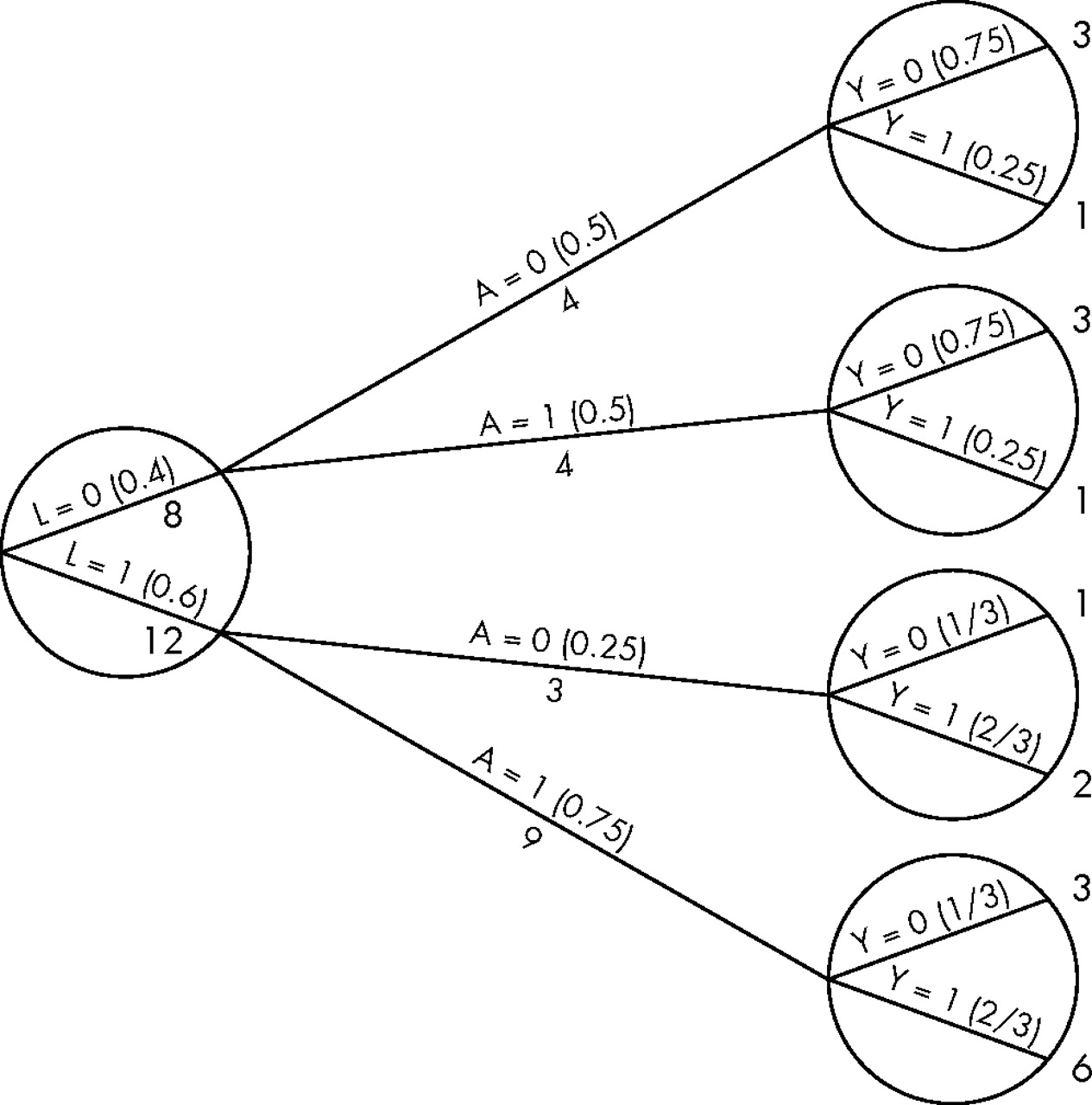
The data in table 1 can be displayed as a tree (fig 1) in which all 20 persons start at the left and progress over time towards the right. The leftmost circle of the tree contains its first branching: eight persons were in non-critical condition (L = 0) and 12 in critical condition (L = 1). The numbers in parentheses are the probabilities of being in non-critical (Pr[L = 0] = 8/20 = 0.4) or critical (Pr[L = 0] = 12/20 = 0.6) condition. Let us follow, for example, the branch L = 0. Of the eight persons in this branch, four were unexposed (A = 0) and four were exposed (A = 1). The conditional probability of being unexposed is Pr[A = 0|L = 0] = 4/8 = 0.5, as shown in parentheses. The conditional probability Pr[A = 1]|L = 0 is 0.5 too. The upper right circle represents that, of the four persons in the branch L = 0,A = 0; 3 survived (Y = 0) and 1 died (Y = 1). That is, Pr[Y = 0|L = 0,A = 0] = 3/4 and Pr[Y = 1|L = 0,A = 0] = 1/4. The other branches of the tree are interpreted analogously. The circles contain the bifurcations defined by non-exposure variables (that is, variables for which no hypothetical intervention needs to be defined). We now use this tree to compute the causal risk ratio Pr[Y_a = 1 = 1]/Pr[Y_a = 0 = 1].

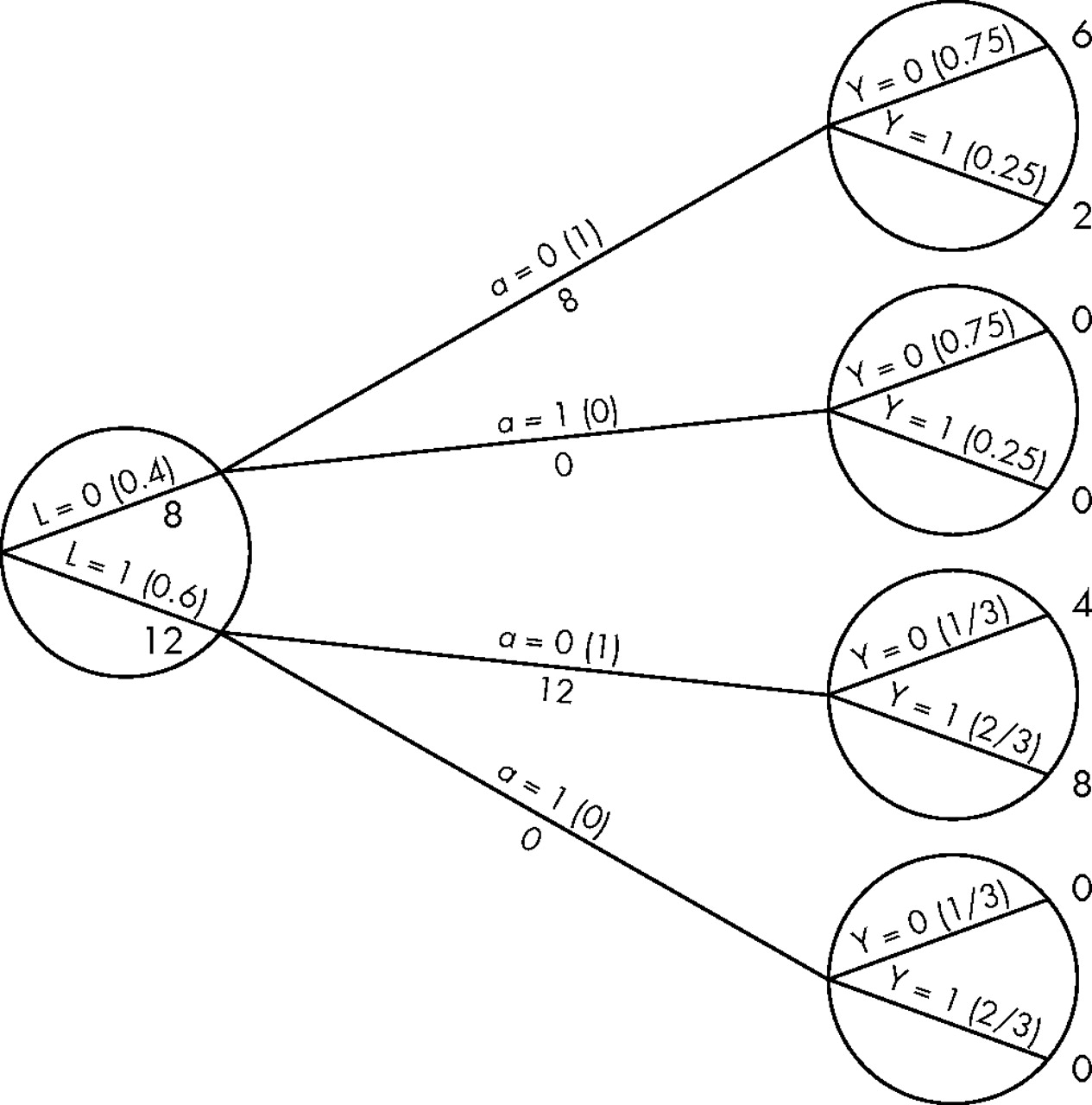
The denominator of the causal risk ratio, Pr[Y_a = 0 = 1], is the counterfactual risk of death had everybody in the population remained unexposed. Let us calculate this risk. In figure 1, four of eight persons with L = 0 were unexposed, and one of them died. How many deaths would have occurred had the eight persons with L = 0 remained unexposed? Two deaths, because if eight persons rather than four persons had remained unexposed, then two deaths rather than one death would have been observed. If the number of persons is multiplied by two, then the number of deaths is also doubled. In figure 1, 3 of 12 persons with L = 1 were unexposed, and two of them died. How many deaths would have occurred had the 12 persons with L = 0 remained unexposed? Eight deaths, or two deaths times four, because 12 is 3×4. That is, if all 8+12 = 20 persons in the population had been unexposed, then 2+8 = 10 would have died. The denominator of the causal risk ratio, Pr[Y_a = 0 = 1], is 10/20 = 0.5. Figure 2 shows the population had everybody remained unexposed (a = 0). Of course, these calculations rely on the assumption that exposed persons with L = 0, had they remained unexposed, would have had the same probability of death as those who actually remained unexposed. This assumption is precisely conditional exchangeability given L = 0.

The numerator of the causal risk ratio Pr[Y_a = 1 = 1] is the counterfactual risk of death had everybody in the population been exposed. Reasoning as in the previous paragraph, this risk is calculated to be also 10/20 = 0.5, under the assumption of conditional exchangeability given L = 1. Figure 3 shows the population had everybody been exposed (a = 1). Combining the results from this and the previous paragraph, the causal risk ratio Pr[Y_a = 1 = 1]/Pr[Y_a = 0 = 1] is equal to 0.5/0.5 = 1 under the assumption of conditional exchangeability We are done.

Let us examine how this method works. Figures 2 and 3 are essentially a simulation of what would have happened had all subjects in the population been unexposed and exposed, respectively. These simulations are correct under the assumption of conditional exchangeability. Both simulations can be pooled to create a hypothetical population in which every person appears both as an exposed and as an unexposed person. This hypothetical population, twice as large as the original population, is often referred to as the pseudo-population. Figure 4 shows the entire pseudo-population. Under conditional exchangeability in the original population, the exposed (a = 1) and the unexposed (a = 0) in the pseudo-population are (unconditionally) exchangeable because they are the same persons under a different exposure level. In other words, there is no confounding in the pseudo-population and the associational risk ratio in the pseudo-population is equal to the causal risk ratio in both the pseudo-population and the original population.

This method is known as inverse probability weighting. To see why, let us look at, say, the four unexposed persons with L = 0 in the population of figure 1. These persons are used to create eight members of the pseudo-population of figure 4. That is, each of them is assigned a weight of 2, which is equal to1/0.5. Figure 1 shows that 0.5 is the conditional probability of staying unexposed given L = 0. Similarly, the nine exposed subjects with L = 1 in figure 1 are used to create 12 members of the pseudo-population. That is, each of them is assigned a weight of 1.33 = 1/0.75. Figure 1 shows that 0.75 is the conditional probability of being exposed given L = 1. Informally, the pseudo-population is created by weighting each person in the population by the inverse of the conditional probability of receiving the exposure that she indeed received. These inverse probability weights are shown in the last column of figure 4.

INVERSE PROBABILITY WEIGHTING VERSUS STANDARDISATION

We have described two analytical approaches to compute causal effects from observational data: standardisation and inverse probability weighting. Both approaches need to supplement observational data with the identifying assumption of conditional exchangeability of the exposed and the unexposed given the measured variables L Investigators can use their expert knowledge to enhance the plausibility of the conditional exchangeability assumption. For example, they can measure many relevant variables (determinants of the exposure that are also risk factors for the outcome), rather than only one variable, as in table 1, and then assume that conditional exchangeability is approximately true within the strata defined by the combination of all those variables L. The validity of the causal inferences depends upon the correctness of this assumption but, no matter how many variables are included in L, there is no way to test that the assumption is correct. That is why causal inference from observational data is a risky task.

Standardisation and inverse probability weighting use the measured data in a different way, but both approaches need data on L to estimate causal effects under the assumption We say that these methods adjust for the measured variables in L. In a slight abuse of language we sometimes say that these methods control for L, but this “analytical control” is quite different from the “physical control” of randomised experiments in which the intervention on exposure assignment ensures the absence of confounding.

Both standardisation and inverse probability weighting yielded the same result (causal risk ratio equal to 1) in our example above. This is no coincidence. In simple settings, standardisation and weighting are exactly equivalent (proof in appendix). On the other hand, the results of standardisation and inverse probability weighting may differ in more complex—and more realistic—settings with multiple, and possibly continuous or time varying, variables. This is so because in complex settings one cannot compute the standardised or weighted risks directly from the table as we did above. For example, to compute the standardised risk, we readily computed Pr[Y = 1|L = l,A = a] and Pr[L = l] by looking at table 1. In a more complex example, we would have needed to use statistical models to estimate the conditional distributions of the variables Y and L. Similarly, to compute the inverse probability weighted risk, we would have needed to use a statistical model to estimate the conditional distribution of the exposure A. In practical applications, the actual estimates from standardisation and inverse probability weighting may differ because they are based on different modelling assumptions.

Standardisation and inverse probability weighting are not the only approaches for causal inference from observational data. Stratification, matching, other propensity score based methods, and instrumental variables are some alternatives. In future articles, we will review the relative advantages and disadvantages of each approach.

In this article we have emphasised that conditional exchangeability is a key condition for causal inference, irrespective of the analytical approach used to compute the causal effect. Additional conditions that are required for causal inference include accurate data measurement, data missing at random, and no interaction between subjects (also known as SUTVA). But these additional conditions differ from (conditional) exchangeability of the exposed and the unexposed in one crucial aspect: they can be violated in observational studies and in randomised experiments, regardless of sample size. Our emphasis on conditional exchangeability derives from its specific relevance to observational data.

BIBLIOGRAPHICAL NOTES

Rubin² described the conditions for estimating causal effects in observational studies with fixed exposures. He also classified missing data as missing completely at random, missing at random, or not missing at random.³ Causal inference can be conceptualised as a missing data problem in which only one counterfactual outcome is observed for each subject. Exchangeability under design 1 implies that the counterfactual outcomes are missing completely at random. Conditional exchangeability under design 2 implies that the counterfactual outcomes are missing at random (given the variables used to define the randomisation probabilities). Under design 3, there is not guarantee that the counterfactual outcomes are missing at random conditionally on the measured covariates. The concepts of identifiability, exchangeability, and confounding were reviewed by Greenland and Robins,⁴ and that of SUTVA by Rubin.⁵

Robins^6,7 established the conditions for estimating causal effects in observational studies with time varying exposures. He also proposed a generalisation of standardisation, the g-formula, to compute the effects of time varying exposures, and proposed the causally structured trees shown in figures 1–5. Inverse probability weighting was first proposed by Horvitz and Thompson in the context of survey sampling.⁸ Robins proposed a class of semiparametric models, marginal structural models, whose parameters can be estimated by inverse probability weighting.⁹ Several real world applications of marginal structural models have been described. See, for example, Cole et al¹⁰ and Choi et al.¹¹

APPENDIX

A.1. THE POSITIVITY CONDITION

We defined the standardised risk for treatment level a as

However, this definition is incomplete because the expression

can only be computed if the conditional probability Pr[Y = 1|A = a,L = l] is well defined; that is, if the conditional probability Pr[A = a|L = l] is greater than zero for all values l that occur in the population. Therefore, the standardised risk is defined as

and is undefined otherwise. The condition “if Pr[A = a|L = l]>0 for all l with Pr[L = l]≠0” is known as the positivity condition and essentially means that the above standardised risk can be computed only if, for each value of the covariate L in the population, there are some subjects that received the exposure level a.

A.2. EQUIVALENCE OF INVERSE PROBABILITY WEIGHTING AND STANDARDISATION

A subject’s inverse probability weight depends on her values of exposure A and covariates in (the vector) L. For example, an exposed subject with L = l receives the weight 1/Pr[A = 1|L = l] whereas an unexposed subject with L = l′ receives the weight 1/Pr[A = 0|L = l′]. We can express these weights using a single expression for all subjects—regardless of their individual exposure and covariate values—by using the probability density function (pdf) of A rather than the probability of A. The conditional pdf of A given L evaluated at the values a and l is represented by f_A|L[a|l] or simply as f[a|l]. For discrete variables A and L, f[a|l] is the conditional probability Pr[A = a|L = l]. As the denominator of the weight for each subject is the conditional density evaluated at the subject’s own values of A and L, it can be expressed as the conditional density evaluated at the random arguments A and L (as compared with the fixed arguments a and l), that is, as f[A|L]. This notation, which already appeared in figure 4, is used to define the inverse probability weights W = 1/f[A|L]. (Note that using probabilities rather than densities would not allow us to present a unified notation for the weights because Pr[A = A|L = L] is not considered proper notation.)

For a dichotomous outcome Y, the risk Pr[Y = 1] is equal to the population mean (or expected value) of Y, E[Y]. Therefore the inverse probability weighted risk for treatment level a is defined as the mean of Y reweighted by 1/f[a|L] in subjects with treatment value A = a. That is, we define to be the inverse probability weighted risk for treatment level a, where the function I = (A = a) takes value 1 for subjects with A = a, and 0 for the others. This is the correct mathematical fomalisation of the inverse probability weighted risk as defined in the main text. It is only well defined when the positivity condition holds, as when positivity does not hold, the undefined ratio occurs in computing the expectation. To intuitively understand why it is not defined when the positivity condition fails, consider figure 1. If there were no exposed subjects (A = 1) with L = 0 it would not be possible to simulate what would have happened had all unexposed subjects been exposed under the assumption of conditional exchangeability. There would be no exposed subjects with L = 0 that could be considered exchangeable with the unexposed subjects with L = 0.

Define the “apparent” inverse probability weighted risk for treatment level a to be This risk is always well defined as its denominator f[A|L] can never be zero. The “apparent” and true inverse probability weighted risks for treatment level a are equal to one another (and to the standardised risk) whenever the positivity condition holds and thus all quantities are well defined. When the positivity condition fails to hold, the “apparent” inverse probability weighted risk for treatment level a is without either a useful statistical or causal interpretation.

It follows that the inverse probability weighted risk can also be defined as

and it is undefined otherwise. We now prove that the inverse probability weighted risk is equal to the standardised risk under the positivity condition. By definition of expected value, and after some simplification,

For the remainder of this appendix, we will assume that the positivity condition holds.

A.3. GENERALISATIONS

A.3.1. Non dichotomous outcome and exposure

The methods described above can be generalised to a non-dichotomous outcome Y by contrasting counterfactual means rather than risks. Let E[Y_a] be the mean of the counterfactual outcome Y_a had all subjects in the population received exposure level a. We now show that the standardised mean and the inverse probability weighted mean are equal to the counterfactual mean E[Y_a].

In general, the standardised mean is where F_Y|A,L[⋅] is the conditional cumulative density function (cdf) of Y given A and L, and F_L(⋅) is the cdf of L. The counterfactual mean equals the standardised mean because F_Y|_A,L[y|a,l] = F_Ya|A,L[y|a,l] by definition of counterfactual outcome, and F_Ya|_A,L[y|a,l] = F_Ya|L[y|l] by conditional exchangeability.

The inverse probability weighted mean equals the standardised mean, as shown above for dichotomous outcomes, and therefore equals the counterfactual mean E[Y_a] under conditional exchangeability. We now present an alternative demonstration of the equality between the inverse probability weighted mean and the counterfactual mean. Some of the material presented in subsequent sections is based upon this demonstration. First note that is equal to by definition of counterfactual outcome. The next steps in the proof are:

The key point is that conditional exchangeability is necessary to interpret both the standardised mean and the inverse probability weighted mean as a counterfactual mean.

The extension to polytomous exposures is straightforward (that is, a can take more than two values). However, this is not the case for continuous exposures because, in realistic scenarios, estimates based on the weights 1/f[A|L] have infinite variance and thus cannot be used. The next section describes generalised weights that can be used with all kinds of exposure variables.

A.3.2. Inverse probability weights

The previous section shows that, using weights W = 1/f[A|L], the inverse probability weighted mean equals the counterfactual mean E[Y_a] under conditional exchangeability. We motivated the use of the weights W as a method for simulating what would have happened had everybody in the population experienced each of the exposure levels. For example, figure 4 displays the number of deaths that would have been observed had everyone been exposed (a = 1) and unexposed (a = 0). The causal risk ratio is then readily calculated as the ratio of the number of deaths under each exposure level. When using the weights W, the pseudo-population is larger than the original population. However, this does not result in a corresponding decrease in the variance because persons in the pseudo-population, unlike those in the original population, are not statistically independent.

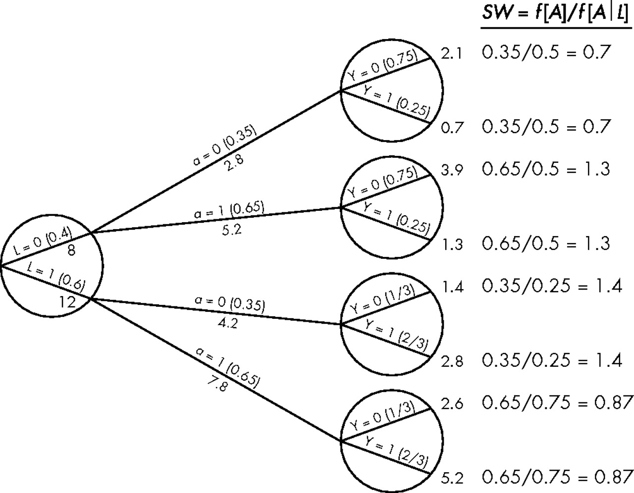
Now suppose that, in contrast with simulating what would have been observed had everyone been exposed and unexposed, we were able to simulate what would have been observed had, say, 65% of the population been exposed and 35% unexposed in every level of L. Under conditional exchangeability, this simulation would provide us with data from a design 1 randomised experiment, and therefore would allow us to compute the causal risk ratio. Using the same argumentation as the one used to construct figure 4, let us simulate what would have happened had 65% of subjects been exposed, and the other 35% unexposed, in the population shown in figure 1. The resulting pseudo-population is displayed in figure 5. In this pseudo-population, the risk in the exposed is and the risk in the unexposed is Therefore the risk ratio is which equals the causal risk ratio computed by using the pseudo-population of figure 4 (see proof below).

The method used to construct the pseudo-population in figure 5 is inverse probability weighting with weights modified to simulate a design 1 randomised experiment. It is easy to check that the pseudo-population in figure 5 can be constructed by applying the weights to the exposed, and to the unexposed in the original population. Because Pr[A = 1] = 0.65 and Pr[A = 0] = 0.35 the numerator of these modified weights is f[A]. We refer to the weights used to construct the pseudo-population in figure 5 as stabilised inverse probability weights SW. When using the weights SW (or in fact any weight with a density, or a function that integrates to 1, in the numerator), the pseudo-population is of the same size as the original population. Also, the weights SW have mean one because

The causal effect can be computed by using either the non-stabilised weights or the stabilised weights More generally, the causal effect can be computed by using weights where g[A] is any function of A that is not a function of L. We now show that the inverse probability weighted mean with weights is equal to the counterfactual mean E[Y_a]. First note that the inverse probability weighted mean using weights 1/f[A|L] can also be expressed as because Similarly, the inverse probability weighted mean using weights can be expressed as which is also equal to the counterfactual mean E[Y_a]. The proof proceeds as in the previous section to show that the numerator and that the denominator Thus, the choice of weights does not affect the consistency of the estimator of causal effect. However, in more complex and realistic settings in which it is necessary to use models for (functions of) the outcome Y given exposure A, the choice of the weights affects the variability of the estimator of causal effect. In these cases weights are preferable over weights because there exist functions g[A] (for example, f[A]) that can be used to construct more efficient estimators of the causal effect (that is estimators with a narrower confidence interval). Also, weights (for example, the stabilised weights SW) can be used for continuous exposures.

A brief note about estimation. We stated that the weighted means and are equal because However, this is not necessarily true when estimating the inverse probability weighted mean in the population by using the average in a sample. Thus the original Horvitz-Thompson estimator and the modified Horvitz-Thompson estimator may yield different estimates in practice. (The “hat” over E indicates that is the sample average, a consistent estimator of the population mean.) The modified Horvitz-Thompson estimator is used to estimate the parameters of marginal structural models.⁹

A.3.3.The causal effect in a subset of the population

We have used standardisation and inverse probability weighting to compute the causal effect of the exposure on the outcome in the entire population. That is, we computed the causal risk ratio Pr[Y_a = 1 = 1]/Pr[Y_a = 0 = 1] that compares the counterfactual risk had everybody in the population of interest been exposed and the counterfactual risk had everybody in the population been unexposed. But investigators may be interested in the causal effect of the exposure in a subset of the population (for example, men, the exposed) rather than in the causal effect in the entire population. When this is the case, standardisation and inverse probability weighting can be easily modified as follows.

Let S be a pre-exposure non-continuous variable (for example, sex). The causal effect in the risk ratio scale in the subset of population subjects with S = s (for example, men) is Pr[Y_a = 1 = 1|S = s]/Pr[Y_a = 0 = 1|S = s] To compute the counterfactual risk Pr[Y_a = 1|S = s] using standardisation (or the counterfactual mean E[Y_a|S = s] using inverse probability weighting), one just needs to restrict the calculations to the subset of subjects in the population with S = s.

Sometimes the investigators want to compute the causal effect in subjects who were actually exposed (or unexposed). For example, the causal risk ratio in the exposed is Pr[Y_a = 1 = 1|A = 1]/Pr[Y_a = 0 = 1|A = 1] or, by definition of counterfactual outcome, Pr[Y = 1|A = 1]/Pr[Y_a = 0 = 1|A = 1]. The causal risk ratio in the exposed is also known as the standardised morbidity, or mortality, ratio (SMR). Unlike for a pre-treatment variable S, one cannot restrict the calculation of the counterfactual risk Pr[Y_a = 0 = 1|A = 1] to the subset of subjects with A = 1 because the subset of exposed subjects has no information to compute the risk under no exposure.

We now describe how to compute the counterfactual risk Pr[Y_a = 1|A = a′] where a≠a′ by using standardisation, and a more general approach to compute the counterfactual mean E[Y_a|A = a′] by using inverse probability weighting.

1. Standardisation

Pr[Y_a = 1|A = a′] is equal to The steps of the proof are

See Miettinen¹² for a discussion of standardised risk ratios.

2. Inverse probability weighting

E[Y_a|A = a′] is equal to the inverse probability weighted mean

with weights . To prove this equality, first note that the numerator is equal to by definition of counterfactual outcome, and that the denominator is equal to Pr[A = a′] The rest of the proof is

If A is dichotomous and we want to estimate the inverse probability weighted risk in the exposed and the unexposed, our results reduce to those of Sato and Matsuyama.¹³

Note that the effect in the exposed (or the unexposed) can be computed under a weaker conditional exchangeability assumption, for one value a only, than that required to compute the effect in the entire population, for all values of a. But the key point is that some form of conditional exchangeability is always necessary for causal inference.